Quantcast
Channel: Cleve’s Corner: Cleve Moler on Mathematics and Computing
Viewing all 337 articles
Browse latest View live

Fibonacci Matrices

$
0
0

Contents

A bug report

MathWorks recently received a bug report involving the matrix

X = [  63245986, 102334155
      102334155, 165580141]
X =

    63245986   102334155
   102334155   165580141

The report claimed that MATLAB computed an inaccurate result for the determinant of X.

format long
detX = det(X)
detX =

   1.524897739291191

The familiar high school formula gives a significantly different result.

detX = X(1,1)*X(2,2) - X(1,2)*X(2,1)
detX =

     2

While checking out the report, I computed the elementwise ratio of the rows of X and discovered an old friend.

ratio = X(2,:)./X(1,:)
ratio =

   1.618033988749895   1.618033988749895

This is $\phi$, the Golden ratio.

phi = (1 + sqrt(5))/2
phi =

   1.618033988749895

So, I decided to investigate further.

Powers of a Fibonacci matrix

Let's call the following 2-by-2 matrix the Fibonacci matrix.

$$F = \pmatrix{0 & 1 \cr 1 & 1}$$

Generate the matrix in MATLAB

F = [0 1; 1 1]
F =

     0     1
     1     1

The elements of powers of $F$ are Fibonacci numbers. Let $f_n$ be the $n$-th Fibanacci number. Then the $n$-th power of $F$ contains three successive $f_n$.

$$F^n = \pmatrix{f_{n-1} & f_n \cr f_n & f_{n+1}}$$

For example

F2 = F*F
F3 = F*F2
F4 = F*F3
F5 = F*F4
F2 =

     1     1
     1     2


F3 =

     1     2
     2     3


F4 =

     2     3
     3     5


F5 =

     3     5
     5     8

The matrix in the bug report is $F^{40}$.

X = F^40
X =

    63245986   102334155
   102334155   165580141

These matrix powers are computed without any roundoff error. Their elements are "flints", floating point numbers whose values are integers.

Determinants

The determinant of $F$ is clearly $-1$. Hence

$$\mbox{det}(F^n) = (-1)^n$$

So det(F^40) should be 1, not 1.5249, and not 2.

Let's examine the computation of determinants using floating point arithmetic. We expect these to be +1 or -1.

det1 = det(F)
det2 = det(F^2)
det3 = det(F^3)
det1 =

    -1


det2 =

     1


det3 =

    -1

So far, so good. However,

det40 = det(F^40)
det40 =

   1.524897739291191

This has barely one digit of accuracy.

What happened?

It is instructive to look at the accuracy of all the determinants.

d = zeros(40,1);
for n = 1:40
   d(n) = det(F^n);
end
format long
d
d =

  -1.000000000000000
   1.000000000000000
  -1.000000000000000
   0.999999999999999
  -0.999999999999996
   1.000000000000000
  -0.999999999999996
   0.999999999999996
  -1.000000000000057
   0.999999999999872
  -0.999999999999943
   0.999999999997726
  -0.999999999998209
   1.000000000000227
  -1.000000000029786
   1.000000000138243
  -0.999999999990905
   1.000000000261935
  -1.000000000591172
   0.999999999999091
  -0.999999996060069
   1.000000003768946
  -0.999999926301825
   0.999999793712050
  -1.000000685962732
   0.999998350307578
  -0.999995890248101
   0.999983831774443
  -0.999970503151417
   1.000005397945643
  -0.999914042185992
   0.999138860497624
  -0.997885793447495
   0.998510751873255
  -0.996874589473009
   0.973348170518875
  -0.989943694323301
   0.873688660562038
  -0.471219316124916
   1.524897739291191

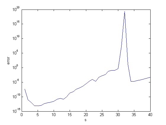
We see that the accuracy deteriorates as n increases. In fact, the number of correct digits is roughly a linear function of n, reaching zero around n = 40.

A log plot of the error

semilogy(abs(abs(d)-1),'.')
set(gca,'ydir','rev')
title('error in det(F^n)')
xlabel('n')
ylabel('error')
axis([0 41 eps 1])

Computing determinants

MATLAB computes determinants as the product of the diagonal elements of the triangular factors resulting from Gaussian elimination.

Let's look at $F^{12}$.

format long e
F12 = F^12
[L,U] = lu(F12)
F12 =

    89   144
   144   233


L =

     6.180555555555555e-01     1.000000000000000e+00
     1.000000000000000e+00                         0


U =

     1.440000000000000e+02     2.330000000000000e+02
                         0    -6.944444444428655e-03

Since $det(L) = -1$,

det(L)
ans =

    -1

we have

det12 = -prod(diag(U))
det12 =

     9.999999999977263e-01

We can see that, for $F^{12}$, the crucial element U(2,2) has lost about 5 significant digits in the elimination and that this is reflected in the accuracy of the determinant.

How about $F^{40}$?

[L,U] = lu(F^40)
det40 = -prod(diag(U))
L =

     6.180339887498949e-01     1.000000000000000e+00
     1.000000000000000e+00                         0


U =

     1.023341550000000e+08     1.655801410000000e+08
                         0    -1.490116119384766e-08


det40 =

     1.524897739291191e+00

The troubling value of 1.5249 from the bug report is a direct result of the subtractive cancellation involved in computing U(2,2). In order for the computed determinant to be 1, the value of U(2,2) should have been

U22 = -1/U(1,1)
U22 =

    -9.771908508943080e-09

Compare U22 with U(2,2). The value of U(2,2) resulting from elimination has lost almost all its accuracy.

This prompts us to check the condition of $F^{40}$.

cond40 = cond(F^40)
cond40 =

   Inf

Well, that's not much help. Something is going wrong in the computation of cond(F^40).

Golden Ratio

There is an intimate relationship between Fibonacci numbers and the Golden Ratio. The eigenvalues of $F$ are $\phi$ and its negative reciprocal.

$$\phi = (1+\sqrt{5})/2$$

$$\bar{\phi} = (1-\sqrt{5})/2$$

format long
phibar = (1-sqrt(5))/2
phi = (1+sqrt(5))/2
eigF = eig(F)
phibar =

  -0.618033988749895


phi =

   1.618033988749895


eigF =

  -0.618033988749895
   1.618033988749895

Because powers of $\phi$ dominate powers of $\bar{\phi}$, it is possible to generate $F^n$ by rounding a scaled matrix of powers of $\phi$ to the nearest integers.

$$F^n = \mbox{round}\left(\pmatrix{\phi^{n-1} & \phi^n \cr \phi^n & \phi^{n+1}}/\sqrt{5}\right)$$

n = 40
F40 = round( [phi^(n-1)  phi^n;  phi^n  phi^(n+1)]/sqrt(5) )
n =

    40


F40 =

    63245986   102334155
   102334155   165580141

Before rounding, the matrix of powers of $\phi$ is clearly singular, so the rounded matrix $F^n$ must be regarded as "close to singular", even though its determinant is $+1$. This is yet another example of the fact that the size of the determinant cannot be a reliable indication of nearness to singularity.

Condition

The condition number of $F$ is the ratio of its singular values, and because $F$ is symmetric, its singular values are the absolute value of its eigenvalues. So

$$\mbox{cond}(F) = \phi/|\bar{\phi}| = \phi^2 = 1+\phi$$

condF = 1+phi
condF =

   2.618033988749895

This agrees with

condF = cond(F)
condF =

   2.618033988749895

With the help of the Symbolic Toolbox, we can get an exact expression for $\mbox{cond}(F^{40}) = \mbox{cond}(F)^{40}$

Phi = sym('(1+sqrt(5))/2');
cond40 = expand((1+Phi)^40)
 
cond40 =
 
(23416728348467685*5^(1/2))/2 + 52361396397820127/2
 

The numerical value is

cond40 = double(cond40)
cond40 =

     5.236139639782013e+16

This is better than the Inf we obtain from cond(F^40). Note that it is more than an order of magnitude larger than 1/eps.

Backward error

J. H. Wilkinson showed us that the L and U factors computing by Gaussian elimination are the exact factors of some matrix within roundoff error of the given matrix. With hindsight and the Symbolic Toolbox, we can find that matrix.

digits(25)
X = vpa(L)*vpa(U)
 
X =
 
[ 63245986.00000000118877885, 102334154.9999999967942319]
[                102334155.0,                165580141.0]
 

Our computed L and U are the actual triangular decomposition of this extended precision matrix. And the determinant of this X is the shaky value that prompted this investigation.

det(X)
 
ans =
 
1.524897739291191101074219
 

The double precision matrix closest to X is precisely $F^{40}$.

double(X)
ans =

    63245986   102334155
   102334155   165580141

Retrospective backward error analysis confirms Wilkinson's theory in this example.

The high school formula

The familiar formula for 2-by-2 determinants

$$\mbox{det}(X) = x_{1,1} x_{2,2} - x_{1,2} x_{2,1}$$

gives +1 or -1 with no roundoff error for all $X = F^n$ with $n < 40$. It fails completely for $n > 40$. The behavior for exactly $n = 40$ is interesting. Set the output format to

format bank

This format allows us to see all the digits generated when converting binary floating point numbers to decimal for printing. Again, let

X = F^40
X =

   63245986.00  102334155.00
  102334155.00  165580141.00

Look at the last digits of these two products.

p1 = X(1,1)*X(2,2)
p2 = X(2,1)*X(1,2)
p1 =

 10472279279564026.00


p2 =

 10472279279564024.00

The 6 at the end of p1 is correct because X(1,1) ends in a 6 and X(2,2) ends in a 1. But the 4 at the end of p2 is incorrect. It should be a 5 because both X(2,1) and X(1,2) end in 5. However, the spacing between floating point numbers of this magnitude is

format short
delta = eps(p2)
delta =

     2

So near p2 only even flints can be represented. In fact, p1 is the next floating point number after p2. The true product of X(2,1) and X(1,2) falls halfway between p1 and p2 and must be rounded to one or the other. The familiar formula cannot possibly produce the correct result.

Historical irony

For many years, the det function in MATLAB would apply the round function to the computed value if all the matrix entries were integers. So, these old versions would have returned exactly +1 or -1 for det(F^n) with n < 40. But they would round det(F^40) to 2. This kind of behavior was the reason we got rid of the rounding.

eig and svd

Let's try to compute eigenvalues and singular values of $F^{40}$.

format long e
eig(F^40)
svd(F^40)
ans =

           0
   228826127


ans =

     2.288261270000000e+08
                         0

Unfortunately, the small eigenvalue and small singular value are completely lost. We know that the small value should be

phibar^40
ans =

     4.370130339181083e-09

But this is smaller than roundoff error in the large value

eps(phi^40)
ans =

     2.980232238769531e-08

Log plots of the accuracy loss in the computed small eigenvalue and the small singular value are similar to our plot for the determinant. I'm not sure how LAPACK computes eigenvalues and singular values of 2-by-2 matrices. Perhaps that can be the subject of a future blog.


Get the MATLAB code

Published with MATLAB® 7.14


Cleve’s Corner, Blogs Edition

$
0
0

This is the debut of the MATLAB Central Blogs edition of Cleve's Corner. For years, I have been writing a column named Cleve's Corner in MathWorks News and Notes. The News and Notes Edition is in an electronic magazine format that is published once or twice a year and that has very specific length and word count constraints. The Blogs Edition can be any length, and I hope to have enough time and interesting material to post a couple of times per month. In fact, I may revive some old newsletter Corners, bring them up to date, and post them here.

I am pleased to be able to use MATLAB and its publish command as my Web authoring environmnent. I have been writing MATLAB code for even longer than I have been writing newsletter columns. Now I can write a blog without learning a new word processor.

I am also pleased to be able to use MathJax to display typeset mathematics. MathJax is, among other things, a LaTex interpreter written in JavaScript that displays mathematics properly in modern Web browsers. Here's an example. My next blog posting will involve a discussion of $\phi$, the Golden Ratio. Now look again at that Greek letter $\phi$. It should have the correct font size and, most importantly, have the same baseline as the surrounding text. This is how $\phi$ would have looked before MathJax. The old $\phi$ is a .png image. Some browsers place it far above the baseline of rest of the sentence. If you zoom in on the page, or print the page, the new $\phi$ should scale and print nicely, but the old $\phi$ will show the pixelation inherent in an sampled image.

MathJax has been developed by Davide Cervone of Union College and at Design Science, the makers of the MathType equation editor. MathJax has the support of SIAM (Society for Industrial and Applied Mathematics), the AMS (American Mathematical Society), the AIP (American Institute of Physics), a few other professional societies, and several publishers. For more about MathJax, see the recent article by Cervone in the AMS Notices.


Get the MATLAB code

Published with MATLAB® 7.14

Biorhythms

$
0
0

Biorhythms were invented over 100 years ago and entered our popular culture in the 1960s. You can still find many Web sites today that offer to prepare personalized biorhythms, or that sell software to compute them. Biorhythms are based on the notion that three sinusoidal cycles influence our lives. The physical cycle has a period of 23 days, the emotional cycle has a period of 28 days, and the intellectual cycle has a period of 33 days. For any individual, the cycles are initialized at birth. All the people on earth born on one particular day share the biorhythm determined by that date.

Contents

Personal biorhythm

I hope you can download the latest version of my biorhythm program from MATLAB Central at this link. If you already happen to have access to the programs from my book "Experiments with MATLAB", you will find an earlier version of biorhythm there. Either of these programs will allow you to compute your own personal biorhythm.

Vectorized plots

Biorhythms are an excellent way to illustrate MATLAB's vector plotting capabilities. Let's start with a column vector of time measured in days.

t = (0:28)';

The first way you might think of to compute the biorhythm for these days is create this array with three columns.

y = [sin(2*pi*t/23) sin(2*pi*t/28) sin(2*pi*t/33)];

Or, we can get fancy by moving the square brackets inside the sin(...) evaluation and, while we're at it, define an anonymous function. This vectorized calculation is the core of our biorhythm function.

bio = @(t) sin(2*pi*[t/23 t/28 t/33]);
y = bio(t);

We're now ready for our first plot. Because t goes from 0 to 28, the 23-day blue curve covers more than its period, the 28-day green curve covers exactly one period, and the 33-day red curve covers less its period.

clf
plot(t,y)
axis tight

Date functions

MATLAB has several functions for computations involving calendars and dates. They are all based on a date number, which is the amount of time, in units of days, since an arbitrary origin in year zero. The current datenum is provided by the function now. I am writing this post on June 10, 2012, and every time I publish it, the value of now changes. Here is the current value.

format compact
format bank
date = now
date =
     735030.87

A readable form of the current date is provided by datestr.

datestr(now)
ans =
10-Jun-2012 20:45:47

The integer part of now is a date number for the entire day. This value is used in biorhythm.

format short
today = fix(now)
today =
      735030

Newborn

With no input arguments, my latest version of biorhythm plots the biorhythm for a baby born four weeks before today. The plot covers the eight week period from the baby's birth until a date four weeks in the future. You can see the three curves all initialized at birth. The blue physical cycle has a 23-day period, so it passes through zero five days before today. The green emotional cycle has a 28-day period, so it hits zero today. And, the red intellectual cycle will be zero five days from today.

biorhythm

Twenty-first Birthday

Let's look at the biorhythm for someone whose 21st birthday is today. The date vector for such a birthday is obtained by subtracting 21 from the first component of today's datevec. This is a pretty unexciting, but typical, biorhythm. All three cycles are near their midpoints. Blue and red peaked about a week ago and green will peak a little more than a week from now.

birthday = datevec(today) - [21 0 0 0 0 0];
biorhythm(birthday)

Rebirth

Does your biorhythm ever start over? Yes, it does, at a time t when t/23, t/28 and t/33 are all integers. Since the three periods are relatively prime, the first such value of t is their product.

tzero = 23*28*33
tzero =
       21252

How many years and days is this?

dpy = 365+97/400         % 365 days/year + 97/400 for leap years.
yzero = fix(tzero/dpy)
dzero = dpy*mod(tzero/dpy,1)
dpy =
  365.2425
yzero =
    58
dzero =
   67.9350

So, your biorhythm starts over when you are 58 years old, about 68 days after your birthday.

biorhythm(today-tzero)

Nearly Perfect Day

Is there ever a perfect day, one where all three cycles reach their maximum at the same time? Well, not quite. That would require a time t when, for p = 23, 28, 33, t/p = n+1/4, where n is an integer. Then sin(2*pi*t/p) would equal sin(pi/2), which is the maximum. But, since the values of p are relatively prime, there is no such value of t. But we can get close. To find the nearly perfect day, look for the maximum value of the sum of the three cycles.

t = (1:tzero)';
y = bio(t);
s = sum(y,2);
top = find(s==max(s))
biorhythm(today-top)
top =
       17003

How old are you on this nearly perfect day?

top/dpy
ans =
   46.5526

So, half-way through your 46th year.

Detail

But the nearly perfect day is not perfection. The three cyles are not quite at their peaks.

bio(top)
ans =
    0.9977    1.0000    0.9989

Let's zoom in to a two day window around top, the location of the maximum sum. Measure time in hours.

clf
t = (-1:1/24:1)';
y = 100*bio(top+t);
plot(24*t,y)
set(gca,'xaxislocation','top','xlim',[-24 24],'xtick',-24:6:24,...
   'ylim',[96.0 100.4])
title(['biorhythms near day ' int2str(top) ', time in hours'])

We can see that the three peaks occur six hours apart. This is the closest we get to perfection, and the only time in the entire 58-year cycle when we get even this close.

Have a good day.


Get the MATLAB code

Published with MATLAB® 7.14

Symplectic Spacewar

$
0
0

This is the probably the first article ever written with the title "Symplectic Spacewar". If I Google that title today, including the double quotes to keep the two words together, I do not get any hits. But as soon as Google notices this post, I should be able to see at least one hit.

Contents

Symplectic

Symplectic is an infrequently used mathematical term that describes objects joined together smoothly. It also has something to do with fish bones. For us, it is a fairly new class of numerical methods for solving certain special types of ordinary differential equations.

Spacewar

Spacewar is now generally recognized as the world's first video game. It was written by Steve "Slug" Russell and some of his buddies at MIT in 1962. Steve was a reseach assistant for Professor John McCarthy, who moved from MIT to Stanford in 1963. Steve came to California with McCarthy, bringing Spacewar with him. I met Steve then and played Spacewar a lot while I was a grad student at Stanford.

Spacewar ran on the PDP-1, Digital Equipment Corporation's first computer. Two space ships, controlled by players using switches on the console, shoot space torpedoes at each other. The space ships and the torpedoes orbit around a central star. Here is a screen shot.

X = imread('http://blogs.mathworks.com/images/cleve/Spacewar1.png');
imshow(X)

And here is a photo, taken at the Vintage Computer Fair in 2006, of Steve and the PDP-1. The graphics display, an analog cathrode ray tube driven by the computer, can be seen over Steve's shoulder. The bank of sense switches is at the base of the console.

X = imread('http://blogs.mathworks.com/images/cleve/Steve_Russell.png');
imshow(X)

A terrific Java web applet, written by Barry and Brian Silverman and Vadim Gerasimov, provides a simulation of PDP-1 machine instructions running Spacewar. It is available here. Their README files explains how to use the keyboard in place of the sense switches. You should start by learning how to turn the spaceship and fire its rockets to avoid being dragged into the star and destroyed.

Circle generator

The gravitational pull of the star causes the ships and torpedos to move in elliptical orbits, like the path of the torpedo in the screen shot. Steve's program needed to compute these trajectories. At the time, there was nothing like MATLAB. Programs were written in machine language, with each line of the program corresponding to a single machine instruction. I don't think there was any floating point arithmetic hardware; floating point was probably done in software. In any case, it was desirable to avoid evaluation of trig functions in the orbit calculations.

The orbit-generating program would have looked something like this.

      x = 0
      y = 32768
   L: plot x y
      load y
      shift right 2
      add x
      store in x
      change sign
      shift right 2
      add y
      store in y
      go to L

What does this program do? There are no trig functions, no square roots, no multiplications or divisions. Everything is done with shifts and additions. The initial value of y, which is $2^{15}$, serves as an overall scale factor. All the arithmetic involves a single integer register. The "shift right 2" command takes the contents of this register, divides it by $2^2$, and discards any remainder.

Notice that the current value of y is used to update x, then this new x is used to update y. This optimizes both instruction count and storage requirements because it is not necessary to save the current x to update y. But, as we shall see, this is also the key to the method's numerical stability.

Original

If the Spacewar orbit generator were written today in MATLAB, it would look something the following. There are two trajectories, with different step sizes. The blue trajectory has h = 1/4, corresponding to "shift right 2". The green trajectory has h = 1/32, corresponding to "shift right 5". We are no longer limited to integer values, so I have changed the scale factor from $2^{15}$ to $1$. The trajectories are not exact circles, but in one period they return to near the starting point. Notice, again, that the current y is used to update x and then the new x is used to update y.

clf
axis(1.5*[-1 1 -1 1])
axis square
bg = 'blue';

for h = [1/4 1/32]
   x = 0;
   y = 1;
   line(x,y,'marker','o','color','k')
   for t = 0:h:2*pi
      line(x,y,'marker','.','color',bg)
      x = x + h*y;
      y = y - h*x;
   end
   bg = [0 2/3 0];
end
title('Original')

Euler's method

An exact circle would be generated by solving this system of ordinary differential equations.

$$\dot{x}_1 = x_2$$

$$\dot{x}_2 = -x_1$$

This can be written in vectorized form as

$$\dot{x} = A x$$

where

$$A = \pmatrix{0 & 1 \cr -1 & 0}$$

The simplest method for computing an approximate numerical solution to this system, Euler's method, is

$$x(t+h) = x(t) + h A x(t)$$

In the vectorized MATLAB code, all components of x are updated together. This causes the trajectories to spiral outward. Decreasing the step size decreases the spiraling rate, but does not eliminate it.

clf
axis(1.5*[-1 1 -1 1])
axis square
bg = 'blue';

A = [0 1; -1 0];
for h = [1/4 1/32]
   x = [0 1]';
   line(x(1),x(2),'marker','o','color','k')
   for t = 0:h:6*pi
      x = x + h*A*x;
      line(x(1),x(2),'marker','.','color',bg)
   end
   bg = [0 2/3 0];
end
title('Euler')

Implicit Euler

The implicit Euler method is intended to illustrate methods for stiff equations. This system is not stiff, but let's try implicit Euler anyway. Implicit methods usually involve the solution of a nonlinear algebraic system at each step, but here the algebraic system is linear, so backslash does the job.

$$(I - h A) \ x(t+h) = x(t)$$

Again, all the components of the numerical solution are updated simultaneously. Now the trajectories spiral inward.

clf
axis(1.5*[-1 1 -1 1])
axis square
bg = 'blue';

I = eye(2);
A = [0 1; -1 0];
for h = [1/4 1/32]
   x = [0 1]';
   line(x(1),x(2),'marker','o','color','k')
   for t = 0:h:6*pi
      x = (I - h*A)\x;
      line(x(1),x(2),'marker','.','color',bg)
   end
   bg = [0 2/3 0];
end
title('Implicit Euler')

Eigenvalues

Eigenvalues are the key to understanding the behavior of these three circle generators. Let's start with the explicit Euler. The trajectories are given by

$$ x(t+h) = E x(t) $$

where

$$ E = I + h A = \pmatrix{1 & h \cr -h & 1} $$

The matrix $E$ is not symmetric. Its eigenvalues are complex, hence the circular behavior. The eigenvalues satisfy

$$ \lambda_1 = \bar{\lambda}_2 $$

$$ \lambda_1 + \lambda_2 = \mbox{trace} (E) = 2 $$

$$ \lambda_1 \cdot \lambda_2 = \mbox{det} (E) = 1 + h^2 $$

The determinant is larger than 1 and the product of the eigenvalues is the determinant, so they must be outside the unit circle. The powers of the eigenvalues grow exponentially and hence so do the trajectories. We can reach this conclusion without actually finding the eigenvalues, even though that would be easy in this case.

The implicit Euler matrix is the inverse transpose of the explicit matrix.

$$ x(t+h) = E^{-T} x(t) $$

The eigenvalues of $E^{-T}$ are the reciprocals of the eigenvalues of $E$, so they are inside the unit circle. Their powers decay exponentially and hence so do the trajectories.

Today, the spacewar circle generator would be called "semi-implicit". Explicit Euler's method is used for one component, and implicit Euler for the other.

$$\pmatrix{1 & 0 \cr h & 1} x(t+h) = \pmatrix{1 & h \cr 0 & 1} x(t)$$

So

$$x(t+h) = S x(h)$$

where

$$S = \pmatrix{1 & 0 \cr h & 1}^{-1} \pmatrix{1 & h \cr 0 & 1} = \pmatrix{1 & h \cr -h & 1-h^2}$$

The eigenvalues satisfy

$$ \lambda_1 + \lambda_2 = \mbox{trace} (S) = 2 - h^2 $$

$$ \lambda_1 \cdot \lambda_2 = \mbox{det} (S) = 1 $$

The key is the determinant. It is equal to 1, so we can conclude (without actually finding the eigenvalues)

$$ |\lambda_1| = |\lambda_2| = 1$$

The powers $\lambda_1^n$ and $\lambda_2^n$ remain bounded for all $n$.

It turns out that if we define $\theta$ by

$$ \cos{\theta} = 1 - h^2/2 $$

then

$$ \lambda_1^n = \bar{\lambda}_2^n = e^{i n \theta} $$

If, instead of an inverse power of 2, the step size $h$ happens to correspond to a value of $\theta$ that is $2 \pi / p$, where $p$ is an integer, then the spacewar circle produces only $p$ discrete points before it repeats itself.

How close does our circle generator come to actually generating circles? The matrix $S$ is not symmetric. Its eigenvectors are not orthogonal. This can be used to show that the generator produces ellipses. As the step size $h$ gets smaller, the ellipses get closer to circles. It turns out that the aspect ratio of the ellipse, which is the ratio of its major axis to its minor axis, is equal to the condition number of the matrix of eigenvectors.

Symplectic Integrators

Symplectic methods for the numerical solution of ordinary differential equations apply to the class of equations derived from conserved quantities known as Hamiltonians. The components of the solution belong to two subsets, $p$ and $q$, and the Hamiltonian is a function of these two components, $H(p,q)$. The differential equations are

$$\dot{p} = \frac{\partial H(p,q)}{\partial q}$$

$$\dot{q} = -\frac{\partial H(p,q)}{\partial p}$$

For our circle generator, $p$ and $q$ are the coordinates $x$ and $y$, and $H$ is one-half the square of the radius.

$$H(x,y) = \textstyle{\frac{1}{2}}(x^2 + y^2)$$

Hamiltonian systems include models based on Newton's Second Law of Motion, $F = ma$. In this case $p$ is the position, $q$ is the velocity, and $H(p,q)$ is the energy.

Symplectic methods are semi-implicit. They extend the idea of using the current value of $q$ to update $p$ and then using the new value of $p$ to update $q$. This makes it possible to conserve the value of $H(p,q)$, to within the order of accuracy of the method. The spacewar circle generator is a first order symplectic method. The radius is constant, to within an accuracy proportional to the step size $h$.

For other examples of symplectic methods, including the n-body problem of orbital mechanics, see the Orbits chapter and the orbits.m program of Experiments with MATLAB. Here is a screen shot showing the inner planets of the solar system.

X = imread('http://blogs.mathworks.com/images/cleve/solar2.png');
imshow(X)

Steve Russell certainly didn't know that his Spacewar was using a symplectic integrator. That term wasn't invented until years later. It is serendipity that the shortest machine language program has the best numerical properties.

References

[1] http://en.wikipedia.org/wiki/Spacewar!, Wikipedia article on Spacewar.

[2] http://en.wikipedia.org/wiki/File:Steve_Russell_and_PDP-1.png, Steve Russell and the Computer History Museum's PDP-1 at the Vintage Computer Fair 2006.


Get the MATLAB code

Published with MATLAB® 7.14

Exponential Growth

$
0
0

What, exactly, is exponential growth? What is e and what does it have to do with exponential growth? A simple MATLAB interactive graphic introduces these concepts.

Contents

Exponential growth.

To most people "exponential growth" simply means "very rapid growth". But, more precisely, a time varying quantity grows expontially if the rate of growth is proportional to size of the quantity itself. The rate can even be negative, in which case it is "exponential decay".

I think that students who have taken calculus in high school or college should understand the mathematical ideas involved in exponential growth, but I'm afraid that most of them don't. When I ask students to tell me the derivative of $t^3$, they can usually respond $3t^2$. When I ask them "why?", they say "take the $3$, put it out in front, and subtract $1$ from the exponent". Finding derivatives is a purely mechanical process, like adding fractions or solving quadratic equations. When I ask for the derivative of $3^t$, some will even apply the same process to get $t 3^{t-1}$. There is no understanding of the relationship between differentiation and rate of change.

A function $f(t)$ is growing exponentially if its growth rate, its derivative, is proportional to the function itself. Perhaps the most important function in all of mathematics is the one where this proportionality constant is equal to one, so the function is its own derivative. Let's discover that function.

Approximate derivative.

We can get numerical values and graphs of derivatives without actually differentiating anything. For our purposes, approximate derivatives based on the notion of rate of change are, in some ways, even preferable to actual derivatives. We just have to pick a small step size $h$, say $h = .0001$. Then the approximate derivative of $f(t)$ is

$$ \dot{f}(t) = \frac{f(t+h)-f(t)}{h} $$

2^t

What do we mean by the function

$$ f(t) = 2^t $$

If $t$ is a positive integer, then $2^t$ is $2$ multiplied by itself $t$ times.

$$ 2^0 = 1, \ \ 2^1 = 2, \ \ 2^2 = 4, ... $$

If $t$ is a negative integer, then $2^t$ is $1/2$ multiplied by itself $|t|$ times.

$$ 2^{-1} = 1/2, \ \ 2^{-2} = 1/4, ... $$

If $t = p/q$ is a rational number, the ratio of two integers, $2^{p/q}$ is the $q$-th root of the $p$-th power of $2$.

$$ 2^{1/2} = \sqrt{2} = 1.4142, \ \ 2^{355/113} = \sqrt[113]{2^{355}} = 8.8250, ... $$

Theoretically, for floating point arithmetic, this is all we need to know. All floating point numbers are ratios of two integers. We do not have to be concerned yet about the definition of $2^t$ for irrational $t$. If MATLAB can compute powers and roots, we can plot the graph of $2^t$.

Interactive interface.

The function expgui is included with the software for the book Experiments with MATLAB. I invite you to download the function and run it. It plots the graph of $a^t$ and its approximate derivative. Here is the code that generates the initial plot, with $a = 2$. You can see that the derivative, in green, has the same shape as the function, in blue. This is exponential growth.

   t = 0:1/64:2;
   h = .0001;

   % Compute y = a^t and its approximate derivative

   a = 2.0;
   y = a.^t;
   ydot = (a.^(t+h) - a.^t)/h;

   % Plot

   plot(t,[y; ydot])

   % Label

   axis([0 2 0 9])
   fs = get(0,'defaulttextfontsize')+2;
   text(0.3,6.0,'a = 2.000','fontsize',fs,'fontweight','bold')
   title('y = a^t','fontsize',fs,'fontweight','bold')
   legend('y','dy/dt','location','northwest')
   xlabel('t')
   ylabel('y')

Animation.

At this point, if you are actually running expgui, you can move the blue line with your mouse, changing the value of $a$. If you don't have MATLAB, or haven't downloaded expgui, you can click on this movie to see a simulation of the animation. I hope you get to move the line yourself with expgui. The tactile experience is much more satisfying that just watching the movie.

pi^t

In case you are not able to run expgui or watch the movie, here is the plot of $\pi^t$ and its approximate derivative.

   a = pi;
   y = a.^t;
   ydot = (a.^(t+h) - a.^t)/h;
   p = get(gca,'children');
   set(p(3),'ydata',y)
   set(p(2),'ydata',ydot)
   set(p(1),'string','a = 3.142')

Finding e.

You should soon see that the graph of the derivative of $a^t$ always has the same shape as the graph of $a^t$ itself. If $a$ is less than $2.7$ the derivative is below the function, while if $a$ is greater than $2.8$ the derivative is above the function. By moving the mouse carefully you can find a value in between where the curves lie on top of each other, The critical value of $a$ is 2.718. You have discovered $e$ and $e^t$, the only function in the world that is equal to its own derivative. And, you didn't have to differentiate anything. Here is the final graph.

   y = exp(t);
   p = get(gca,'children');
   set(p(3),'ydata',y)
   set(p(2),'ydata',y)
   set(p(1),'string','a = 2.718')

e^t

In contrast to its equally famous cousin, $\pi$, the actual numerical value of $e$ is not so important. It's the function $e^t$, or exp(t) as it's known in MATLAB, that is fundamental. If you ever need to know the value of $e$, you can always use

format long
e = exp(1)
e =

   2.718281828459046

It's pretty easy to memorize the first ten significant figures.

fprintf('e = %12.9f\n',e)
e =  2.718281828


Get the MATLAB code

Published with MATLAB® 7.14

Symmetric Pair Decomposition

$
0
0

An esoteric fact about matrices is that any real matrix can be written as the product of two symmetric matrices. I've known about this fact for years, but never seriously explored the computational aspects. So I'm using this post to clarify my own understanding of what I'll call the symmetric pair decomposition. It turns out that there are open questions. I don't think we know how to reliably compute the factors. But I also have to admit that, even if we could compute them, I don't know of any practical use.

Contents

Theorem

Not many people know about this theorem.

Theorem: Any real matrix is equal to the product of two real symmetric matrices.

Almost Proof

At first glance this theorem has nothing to do with eigenvalues. But here is the beginning of a proof, and a possible algorithm. Suppose that a real matrix $A$ has real, distinct eigenvalues. Then it can be diagonalized by the matrix $V$ of its eigenvectors.

$$A = V D V^{-1}$$

Because we are assuming there are no multiple eigenvalues, the matrix $V$ exists and is nonsingular, and the matrix $D$ is real and diagonal. Let

$$S_1 = V D V^T$$

$$S_2 = V^{-T} V^{-1}$$

Then $S_1$ and $S_2$ are real, symmetric, and their product is

$$S_1 S_2 = A$$

This argument is not a proof. It just makes the theorem plausible. The challenge comes when the matrix has repeated eigenvalues and lacks a full set of eigenvectors, so it cannot be diagonalized. A complete proof would transform the matrix to its Rational Canonical Form or its Jordan Canonical form and construct explicit symmetric factors for the blocks in the canonical form.

Degrees of Freedom

If $A$ is $n$ -by- $n$ and

$$A = S_1 S_2$$

where each of the symmetric matrices has $n(n+1)/2$ independent elements, then this is $n^2$ nonlinear equations in $n^2+n$ unknowns. It looks like there could be an $n$-parameter family of solutions. In my almost proof, each eigenvector is determined only up to a scale factor. These $n$ scale factors show up in $S_1$ and $S_2$ in complicated, nonlinear ways. I suspect that allowing complex scale factors parameterizes the complete set of solutions, but I'm not sure.

Moler's Rules

My two Golden Rules of computation are:

  • The hardest things to compute are things that do not exist.
  • The next hardest things to compute are things that are not unique.

For the symmetric pair decomposition, our obscure theorem says the decomposition exists, but the degrees of freedom observation says it is probably not unique. Worse yet, the only algorithm we have requires a full set of eigenvectors, which may not exist. We will have to worry about these things.

LU Decomposition

The most important decomposition in numerical linear algebra, the one we use to solve systems of simultaneous linear equations, is the LU decomposition. It expresses a permuted matrix as the product of two triangular factors.

$$P A = L U$$

The permutation matrix $P$ gives us existence and numerical stability. Putting ones on the diagonal of $L$ eliminates $n$ degrees of freedom and give us uniqueness.

Magic Square

Our first example involves one of my favorite matrices.

A = magic(3)
A =

     8     1     6
     3     5     7
     4     9     2

Use the Symbolic Toolbox to compute the eigenvalues and vectors exactly.

[V,D] = eig(sym(A))
 
V =
 
[ (2*6^(1/2))/5 - 7/5, - (2*6^(1/2))/5 - 7/5, 1]
[ 2/5 - (2*6^(1/2))/5,   (2*6^(1/2))/5 + 2/5, 1]
[                   1,                     1, 1]
 
 
D =
 
[ -2*6^(1/2),         0,  0]
[          0, 2*6^(1/2),  0]
[          0,         0, 15]
 

Notice that the elements of V and D involve $\sqrt{6}$ and so are irrational. Now let

S1 = simplify(V*D*V')
S2 = simplify(inv(V*V'))
 
S1 =
 
[ 1047/25, -57/25,  27/5]
[  -57/25, 567/25, 123/5]
[    27/5,  123/5,    15]
 
 
S2 =
 
[ 3/16, 1/12,  1/16]
[ 1/12,  1/2,  -1/4]
[ 1/16, -1/4, 25/48]
 

The $\sqrt{6}$ has disappeared. You can see that S1 and S2 are symmetric, have rational entries, and, as advertised, their product is

Product = S1*S2
 
Product =
 
[ 8, 1, 6]
[ 3, 5, 7]
[ 4, 9, 2]
 

Let's play with the scale factors a bit. I particularly like

V(:,3) = 2
S1 = simplify(V*D*V')/48
S2 = 48*simplify(inv(V*V'))
 
V =
 
[ (2*6^(1/2))/5 - 7/5, - (2*6^(1/2))/5 - 7/5, 2]
[ 2/5 - (2*6^(1/2))/5,   (2*6^(1/2))/5 + 2/5, 2]
[                   1,                     1, 2]
 
 
S1 =
 
[ 181/100,  89/100, 21/20]
[  89/100, 141/100, 29/20]
[   21/20,   29/20,   5/4]
 
 
S2 =
 
[  5,   0,  -1]
[  0,  20, -16]
[ -1, -16,  21]
 

Now S1 has decimal fraction entries, and S2 has integer entries, including two zeros. Let's leave the symbolic world.

S1 = double(S1)
S2 = double(S2)
Product = S1*S2
S1 =

    1.8100    0.8900    1.0500
    0.8900    1.4100    1.4500
    1.0500    1.4500    1.2500


S2 =

     5     0    -1
     0    20   -16
    -1   -16    21


Product =

     8     1     6
     3     5     7
     4     9     2

I can't promise to get such pretty results with other examples.

Nearly Defective

Suppose I want to compute the symmetric pair decomposition of this perturbation of a Jordan block.

e = sym('e','positive');
A = [2 1 0 0; 0 2 1 0; 0 0 2 1; e 0 0 2]
 
A =
 
[ 2, 1, 0, 0]
[ 0, 2, 1, 0]
[ 0, 0, 2, 1]
[ e, 0, 0, 2]
 

Here is the eigenvalue decomposition. The vectors have been scaled so that the last component is equal to 1. The eigenvalues are located on a circle in the complex plane centered at 2, with a radius of e^(1/4), which is the signature of an eigenvalue of multiplicity 4.

[V,D] = eig(A);
V = simplify(V)
D = simplify(D)
 
V =
 
[ -i/e^(3/4),  i/e^(3/4), 1/e^(3/4), -1/e^(3/4)]
[ -1/e^(1/2), -1/e^(1/2), 1/e^(1/2),  1/e^(1/2)]
[  i/e^(1/4), -i/e^(1/4), 1/e^(1/4), -1/e^(1/4)]
[          1,          1,         1,          1]
 
 
D =
 
[ 2 - e^(1/4)*i,             0,           0,           0]
[             0, e^(1/4)*i + 2,           0,           0]
[             0,             0, e^(1/4) + 2,           0]
[             0,             0,           0, 2 - e^(1/4)]
 

Here is the symmetric pair decomposition resulting from this eigenvalue decomposition.

S1 = simplify(V*D*V.')
S2 = simplify(inv(V*V.'))
 
S1 =
 
[   0, 4/e, 8/e, 0]
[ 4/e, 8/e,   0, 0]
[ 8/e,   0,   0, 4]
[   0,   0,   4, 8]
 
 
S2 =
 
[   0,   0, e/4,   0]
[   0, e/4,   0,   0]
[ e/4,   0,   0,   0]
[   0,   0,   0, 1/4]
 

Well, this sort of does the job. S1 and S2 are symmetric and their product is equal to A.

Product = S1*S2
 
Product =
 
[ 2, 1, 0, 0]
[ 0, 2, 1, 0]
[ 0, 0, 2, 1]
[ e, 0, 0, 2]
 

But I am worried that the factors are very badly scaled. As I make e smaller, the large elements in S1 get larger, and the small elements in S2 get smaller. The decomposition breaks down.

A Better Decomposition

A better decomposition is just a rotation. These two matrices are symmetric and their product is A.

S2 = sym(rot90(eye(size(A))))
S1 = A/S2
Product = S1*S2
 
S2 =
 
[ 0, 0, 0, 1]
[ 0, 0, 1, 0]
[ 0, 1, 0, 0]
[ 1, 0, 0, 0]
 
 
S1 =
 
[ 0, 0, 1, 2]
[ 0, 1, 2, 0]
[ 1, 2, 0, 0]
[ 2, 0, 0, e]
 
 
Product =
 
[ 2, 1, 0, 0]
[ 0, 2, 1, 0]
[ 0, 0, 2, 1]
[ e, 0, 0, 2]
 

Can I reproduce this decomposition by rescaling the eigenvectors? Here is code that uses the symbolic solve function to compute new scale factors. If you want to see how it works, download this M-file using the link at the end of this post, remove the semicolons in this section, and run or publish it again.

s = sym('s',[4,1]);
V = V*diag(s);
T = simplify(inv(V*V.'));
soln = solve(T(:,1)-S2(:,1));
s = [soln.s1(1); soln.s2(1); soln.s3(1); soln.s4(1)]
 
s =
 
  (e^(3/4)*i)^(1/2)/2
 (-e^(3/4)*i)^(1/2)/2
            e^(3/8)/2
   (-e^(3/4))^(1/2)/2
 

These scale factors are complex numbers with magnitude e^(3/8)/2. Let's rescale the eigenvectors. Of course, the eigenvalues don't change.

[V,D] = eig(A);
V = simplify(V*diag(s))
 
V =
 
[ -(-1)^(3/4)/(2*e^(3/8)),    (-1)^(1/4)/(2*e^(3/8)), 1/(2*e^(3/8)), -i/(2*e^(3/8))]
[ -(-1)^(1/4)/(2*e^(1/8)), -1/(-1)^(1/4)/(2*e^(1/8)), 1/(2*e^(1/8)),  i/(2*e^(1/8))]
[  ((-1)^(3/4)*e^(1/8))/2,   -((-1)^(1/4)*e^(1/8))/2,     e^(1/8)/2, -(e^(1/8)*i)/2]
[  ((-1)^(1/4)*e^(3/8))/2,  (1/(-1)^(1/4)*e^(3/8))/2,     e^(3/8)/2,  (e^(3/8)*i)/2]
 

Now these eigenvectors produce the same stable decomposition as the rotation.

S1 = simplify(V*D*V.')
S2 = simplify(inv(V*V.'))
 
S1 =
 
[ 0, 0, 1, 2]
[ 0, 1, 2, 0]
[ 1, 2, 0, 0]
[ 2, 0, 0, e]
 
 
S2 =
 
[ 0, 0, 0, 1]
[ 0, 0, 1, 0]
[ 0, 1, 0, 0]
[ 1, 0, 0, 0]
 

Can carefully choosing the scaling of the eigenvectors be the basis for a sound numerical algorithm? I doubt it. We're still trying to compute something that is not unique, using factors that almost do not exist. It's pretty shaky.


Get the MATLAB code

Published with MATLAB® 7.14

Friday the 13th

$
0
0

We all know that Friday the 13th is unlucky, but is it unlikely?

Contents

Year 2012

I plan to post this article during the second week of July, 2012. The Friday in this week is a Friday the 13th, the third we've had so far this year. There were also ones in January and April. That seems like a lot. How often do we have three Friday the 13ths in the first seven months of a year? Well, it's not all that often. It usually happens only once every 28 years. The next time will be the year 2040. But sometimes, around the turn of centuries, it happens twice in 12 years. I mention all this to establish that our calendar does not have a simple periodic behavior. By the way, not to worry, after this week, it will be 14 months until the next Friday the 13th, in September, 2013.

Friday the 13th

Which brings us to the central topic of this post:

  • What is the probability that the 13th of a month falls on a Friday?

An obvious response is

  • Easy question, the probability is 1/7.

After all, there are seven days in a week and the 13th of a month is equally likely to fall on any one of them. Well, as we shall see, that's close, but not exactly right.

Calendars and Leap Years

Leap years make our calendar a nontrivial mathematical object. The leap year rule can be implemented by this anonymous function.

leapyear = @(y) mod(y,4)==0 & mod(y,100)~=0 | mod(y,400)==0;

This says that leap years happen every four years, except the turn of a century not divisible by 400 is skipped. Try a few year numbers.

y = [2012 2013 2000 2100]';
disp([y leapyear(y)])
        2012           1
        2013           0
        2000           1
        2100           0

So, this year is a leap year, next year is not, 2000 was a leap year, 2100 is not.

The leap year rule implies that our calendar has a period of 400 years. The calendar from 1601 to 2000 is being reused from 2001 to 2400. (Except the Gregorian calendar had not been invented in 1601, so I'm talking about the calendar that would have been used back then if they could have used today's calendar, but never mind.)

In a 400 year period, there are 97 leap years, 4800 months, 20871 weeks, and 146097 days. So the average number of days in a calendar year is not 365.25, but

format short
dpy = 365+97/400
dpy =

  365.2425

We can compute the probability that the 13th of a month is a Friday by counting how many times that happens in 4800 months. The correct probability is then that count divided by 4800. Since 4800 is not divisible by 7, the probability does not reduce to 1/7.

Clock

MATLAB has a number of functions for doing computations involving calendars and dates. Many of these functions are in the MATLAB Toolbox, but some of the more specialized ones are in the Finance Toolbox. We encountered a few of these functions in my blog about biorhythms. The basis for all the functions is clock, which reads the system's clock and returns a 6-element vector

  [year, month, date, hour, minute, seconds]

The first five elements have integer values. The sixth element has a fractional part whose accuracy depends upon the computer's internal clock. Here is the output generated when I publish this blog.

c = clock;
fprintf('clock = [ %4d %4d %5d %5d %5d %8.3f ]\n',c)
clock = [ 2012    7     5    11    53   14.258 ]

Datenum

The datenum function facilitates computations involving calendars by collapsing the clock vector into one value, the serial date number. This value is the number of days, and fractions of a day, since a reference time 20 centuries ago when clock would have been all zeros. Here are a couple of examples of the use of datenum. If you run this code yourself, your results should be different.

t = now;
fprintf('current_date_number = %10.3f\n',t)
date_string = datestr(t)
tday = fix(t)
tday_string = datestr(tday)
[week_day,week_day_name] = weekday(tday)
current_date_number = 735055.495

date_string =

05-Jul-2012 11:53:14


tday =

      735055


tday_string =

05-Jul-2012


week_day =

     5


week_day_name =

Thu

Calendar number

The calendar for any year is determined by two pieces of information, the weekday of January 1st and whether or not the year is a leap year. So we need only 14 calendars. We could number all possible calendars, with the units digit specifying the starting week day and the tens digits indicating leap years. The 14 numbers would be [1:7 11:17].

calendar_number = @(y) weekday(datenum(y,1,1)) + 10*leapyear(y);

If the calendar industry used this numbering scheme, here are the calendars you would need for the next 21 years.

y = (2012:2032)';
disp([y calendar_number(y)])
        2012          11
        2013           3
        2014           4
        2015           5
        2016          16
        2017           1
        2018           2
        2019           3
        2020          14
        2021           6
        2022           7
        2023           1
        2024          12
        2025           4
        2026           5
        2027           6
        2028          17
        2029           2
        2030           3
        2031           4
        2032          15

Friday the 13th is likely

We are now ready to use the weekday function to count the number of times in a 400-year calendar cycle that the 13th of a month occurs on each of the various days of the week.

c = zeros(1,7);
for y = 1601:2000
   for m = 1:12
      d = datenum([y,m,13]);
      w = weekday(d);
      c(w) = c(w) + 1;
   end
end
c
c =

   687   685   685   687   684   688   684

A bar graph, with a line at a probability of 1/7, and week day axis labels.

bar(c)
axis([0 8 680 690])
avg = 4800/7;
line([0 8], [avg avg],'linewidth',4,'color','black')
set(gca,'xticklabel',{'Su','M','Tu','W','Th','F','Sa'})

The probability for Friday is

p = c(6)/4800;
fprintf('p = %8.6f\n',p)
fprintf('1/7 = %8.6f\n',1/7)
p = 0.143333
1/7 = 0.142857

So, the 13th of a month is more likely to occur on Friday that any other day of the week. Only slightly more likely, I admit, but still ...


Get the MATLAB code

Published with MATLAB® 7.14

Splines and Pchips

$
0
0

MATLAB has two different functions for piecewise cubic interpolation, spline and pchip. Why are there two? How do they compare?

Contents

Data

Here is the data that I will use in this post.

x = 1:6
y = [16 18 21 17 15 12]
x =

     1     2     3     4     5     6


y =

    16    18    21    17    15    12

Here is a plot of the data.

set(0,'defaultlinelinewidth',2)
clf
plot(x,y,'-o')
axis([0 7 7.5 25.5])
title('plip')

plip

With line type '-o', the MATLAB plot command plots six 'o's at the six data points and draws straight lines between the points. So I added the title plip because this is a graph of the piecewise linear interpolating polynomial. There is a different linear function between each pair of points. Since we want the function to go through the data points, that is interpolate the data, and since two points determine a line, the plip function is unique.

The PCHIP Family

A PCHIP, a Piecewise Cubic Hermite Interpolating Polynomial, is any piecewise cubic polynomial that interpolates the given data, AND has specified derivatives at the interpolation points. Just as two points determine a linear function, two points and two given slopes determine a cubic. The data points are known as "knots". We have the y-values at the knots, so in order to get a particular PCHIP, we have to somehow specify the values of the derivative, y', at the knots.

Consider these two cubic polynomials in $x$ on the interval $1 \le x \le 2$ . These functions are formed by adding cubic terms that vanish at the end points to the linear interpolatant. I'll tell you later where the coefficients of the cubics come from.

$$ s(x) = 16 + 2(x-1) + \textstyle{\frac{49}{18}}(x-1)^2(x-2) - \textstyle{\frac{89}{18}}(x-1)(x-2)^2 $$

$$ p(x) = 16 + 2(x-1) + \textstyle{\frac{2}{5}}(x-1)^2(x-2) - \textstyle{\frac{1}{2}}(x-1)(x-2)^2 $$

These functions interpolate the same values at the ends.

$$ s(1) = 16, \ \ \ s(2) = 18 $$

$$ p(1) = 16, \ \ \ p(2) = 18 $$

But they have different first derivatives at the ends. In particular, $s'(1)$ is negative and $p'(1)$ is positive.

$$ s'(1) = - \textstyle{\frac{53}{18}}, \ s'(2) = \textstyle{\frac{85}{18}} $$

$$ p'(1) = \textstyle{\frac{3}{2}}, \ \ \ p'(2) = \textstyle{\frac{12}{5}} $$

Here's a plot of these two cubic polynomials. The magenta cubic, which is $p(x)$, just climbs steadily from its initial value to its final value. On the other hand, the cyan cubic, which is $s(x)$, starts off heading in the wrong direction, then has to hurry to catch up.

x = 1:1/64:2;
s = 16 + 2*(x-1) + (49/18)*(x-1).^2.*(x-2) - (89/18)*(x-1).*(x-2).^2;
p = 16 + 2*(x-1) + (2/5)*(x-1).^2.*(x-2) - (1/2)*(x-1).*(x-2).^2;

clf
axis([0 3 15 19])
box on
line(x,s,'color',[0 3/4 3/4])
line(x,p,'color',[3/4 0 3/4])
line(x(1),s(1),'marker','o','color',[0 0 3/4])
line(x(end),s(end),'marker','o','color',[0 0 3/4])

If we piece together enough cubics like these to produce a piecewise cubic that interpolates many data points, we have a PCHIP. We could even mix colors and still have a PCHIP. Clearly, we have to be specific when it comes to specifying the slopes.

One possibility that might occur to you briefly is to use the slopes of the lines connecting the end points of each segment. But this choice just produces zeros for the coefficients of the cubics and leads back to the piecewise linear interpolant. After all, a linear function is a degenerate cubic. This illustrates the fact that the PCHIP family includes many functions.

spline

By far, the most famous member of the PCHIP family is the piecewise cubic spline. All PCHIPs are continuous and have a continuous first derivative. A spline is a PCHIP that is exceptionally smooth, in the sense that its second derivative, and consequently its curvature, also varies continuously. The function derives its name from the flexible wood or plastic strip used to draw smooth curves.

Starting about 50 years ago, Carl de Boor developed much of the basic theory of splines. He wrote a widely adopted package of Fortran software, and a widely cited book, for computations involving splines. Later, Carl authored the MATLAB Spline Toolbox. Today, the Spline Toolbox is part of the Curve Fitting Toolbox.

When Carl began the development of splines, he was with General Motors Research in Michigan. GM was just starting to use numerically controlled machine tools. It is essential that automobile parts have smooth edges and surfaces. If the hood of a car, say, does not have continuously varying curvature, you can see wrinkles in the reflections in the show room. In the automobile industry, a discontinuous second derivative is known as a "dent".

The requirement of a continuous second derivative leads to a set of simultaneous linear equations relating the slopes at the interior knots. The two end points need special treatment, and the default treatment has changed over the years. We now choose the coefficients so that the third derivative does not have a jump at the first and last interior knots. Single cubic pieces interpolate the first three, and the last three, data points. This is known as the "not-a-knot" condition. It adds two more equations to set of equations at the interior points. If there are n knots, this gives a well-conditioned, almost symmetric, tridiagonal $n$ -by- $n$ linear system to solve for the slopes. The system can be solved by the sparse backslash operator in MATLAB, or by a custom, non-pivoting tridiagonal solver. (Other end conditions for splines are available in the Curve Fitting Toolbox.)

As you probably realized, the cyan function $s(x)$ introduced above, is one piece of the spline interpolating our sample data. Here is a graph of the entire function, produced by interpgui from NCM, Numerical Computing with MATLAB.

x = 1:6;
y = [16 18 21 17 15 12];
interpgui(x,y,3)

sppchip

I just made up that name, sppchip. It stands for shape preserving piecewise cubic Hermite interpolating polynomial. The actual name of the MATLAB function is just pchip. This function is not as smooth as spline. There may well be jumps in the second derivative. Instead, the function is designed so that it never locally overshoots the data. The slope at each interior point is taken to be a weighted harmonic mean of the slopes of the piecewise linear interpolant. One-sided slope conditions are imposed at the two end points. The pchip slopes can be computed without solving a linear system.

pchip was originally developed by Fred Fritsch and his colleagues at Lawrence Livermore Laboratory around 1980. They described it as "visually pleasing". Dave Kahaner, Steve Nash and I included some of Fred's Fortran subroutines in our 1989 book, Numerical Methods and Software. We made pchip part of MATLAB in the early '90s.

Here is a comparison of spline and pchip on our data. In this case the spline overshoot on the first subinterval is caused by the not-a-knot end condition. But with more data points, or rapidly varying data points, interior overshoots are possible with spline.

interpgui(x,y,3:4)

spline vs. pchip

Here are eight subplots comparing spline and pchip on a slightly larger data set. The first two plots show the functions $s(x)$ and $p(x)$. The difference between the functions on the interior intervals is barely noticeable. The next two plots show the first derivatives. You can see that the first derivative of spline, $s'(x)$, is smooth, while the first derivative of pchip, $p'(x)$, is continuous, but shows "kinks". The third pair of plots are the second derivatives. The spline second derivative $s''(x)$ is continuous, while the pchip second derivative $p''(x)$ has jumps at the knots. The final pair are the third derivatives. Because both functions are piecewise cubics, their third derivatives, $s'''(x)$ and $p'''(x)$, are piecewise constant. The fact that $s'''(x)$ takes on the same values in the first two intervals and the last two intervals reflects the "not-a-knot" spline end conditions.

splinevspchip

Locality

pchip is local. The behavior of pchip on a particular subinterval is determined by only four points, the two data points on either side of that interval. pchip is unaware of the data farther away. spline is global. The behavior of spline on a particular subinterval is determined by all of the data, although the sensitivity to data far away is less than to nearby data. Both behaviors have their advantages and disadvantages.

Here is the response to a unit impulse. You can see that the support of pchip is confined to the two intervals surrounding the impulse, while the support of spline extends over the entire domain. (There is an elegant set of basis functions for cubic splines known as B-splines that do have compact support.)

x = 1:8;
y = zeros(1,8);
y(4) = 1;
interpgui(x,y,3:4)

interp1

The interp1 function in MATLAB, has several method options. The 'linear', 'spline', and 'pchip' options are the same interpolants we have been discussing here. We decided years ago to make the 'cubic' option the same as 'pchip' because we thought the monotonicity property of pchip was generally more desirable than the smoothness property of spline.

The 'v5cubic' option is yet another member of the PCHIP family, which has been retained for compatibility with version 5 of MATLAB. It requires the x's to be equally spaced. The slope of the v5 cubic at point $x_n$ is $(y_{n+1} - y_{n-1})/2$. The resulting piecewise cubic does not have a continuous second derivative and it does not always preserve shape. Because the abscissa are equally spaced, the v5 cubic can be evaluated quickly by a convolution operation.

Here is our example data, modified slightly to exaggerate behavior, and interpgui modified to include the 'v5cubic' option of interp1. The v5 cubic is the black curve between spline and pchip.

x = 1:6;
y = [16 18 21 11 15 12];
interpgui_with_v5cubic(x,y,3:5)

Resources

A extensive collection of tools for curve and surface fitting, by splines and many other functions, is available in the Curve Fitting Toolbox.

doc curvefit

"NCM", Numerical Computing with MATLAB, has more mathematical details. NCM is available online. Here is the interpolation chapter. Here is interpgui. SIAM publishes a print edition.

Here are the script splinevspchip.m and the modified version of interpgui interpgui_with_v5cubic.m that I used in this post.


Get the MATLAB code

Published with MATLAB® 7.14


A Balancing Act for the Matrix Exponential

$
0
0

I have been interested in the computation of the matrix exponential, $e^A$, for a long time. A recent query from a user provides a provocative example.

Contents

Nineteen Dubious Ways

In 1978, Charlie Van Loan and I published a paper in SIAM Review entitled "Nineteen Dubious Ways to Compute the Exponential of a Matrix". The paper does not pick a "best of the 19", but cautiously suggests that the "scaling and squaring" algorithm might be OK. This was about the time I was tinkering with the first MATLAB and consequently every version of MATLAB has had an expm function, based on scaling and squaring. The SIAM Review paper proved to be very popular and in 2003 we published a followup, "Nineteen Dubious Ways ..., Twenty-Five Years Later". A PDF is available from Charlie's web site.

Our colleague Nick Higham reconsided the matrix exponential in 2005. Nick did a careful error analysis of scaling and squaring, improved the efficiency of the algorithm, and wrote a paper for the SIAM Journal on Numerical Analysis, "The scaling and squaring method for the matrix exponential revisited". A PDF is available from the University of Manchester's web site. The current version of expm in MATLAB is Nick's implementation of scaling and squaring.

A more recent review of Nick's work on the matrix exponential is provided by these slides for a talk he gave at a meeting in Rome in 2008.

A Query from a User

A few weeks ago, MathWorks Tech Support received a query from a user about the following matrix. Note that the elements of A range over 18 orders of magnitude.

format long g
a = 2e10;
b = 4e8/6;
c = 200/3;
d = 3;
e = 1e-8;
A = [0 e 0; -(a+b) -d a; c 0 -c]
A =

                         0                     1e-08                         0
         -20066666666.6667                        -3               20000000000
          66.6666666666667                         0         -66.6666666666667

The computed matrix exponential has huge elements.

E = expm(A)
E =

       1.7465684381715e+17         -923050477.783131     -1.73117355055901e+17
     -3.07408665108297e+25      1.62463553675545e+17      3.04699053651329e+25
      1.09189154376804e+17         -577057840.468934     -1.08226721572342e+17

The report claimed that the right answer, obtained from a MATLAB competitor, differs from E by many orders of magnitude.

[  0.446849, 1.54044*10^-9, 0.462811,
  -5.74307*10^6, -0.015283, -4.52654*10^6
   0.447723, 1.5427*10^-9, 0.463481]
ans =

                  0.446849               1.54044e-09                  0.462811
                  -5743070                 -0.015283                  -4526540
                  0.447723                1.5427e-09                  0.463481

Symbolic

Let's generate the symbolic representation of A.

a = sym(2e10);
b = sym(4e8)/6;
c = sym(200)/3;
d = sym(3);
e = sym(1e-8);
S = [0 e 0; -(a+b) -d a; c 0 -c]
 
S =
 
[              0, 1/100000000,           0]
[ -60200000000/3,          -3, 20000000000]
[          200/3,           0,      -200/3]
 

Now have the Symbolic Toolbox compute the matrix exponential, then convert the result to floating point. We can regard this as the "right answer". We see that it agrees with the user's expectations.

X = real(double(expm(S)))
X =

         0.446849468283175      1.54044157383952e-09         0.462811453558774
         -5743067.77947947       -0.0152830038686819         -4526542.71278401
         0.447722977849494      1.54270484519591e-09         0.463480648837651

Classic MATLAB

I ran my old Fortran MATLAB from 1980. Here is the output. It got the right answer.

% <>
% A = <0 e 0; -(a+b) -d a; c 0 -c>
%
%  A     =
%
%     0.000000000000000D+00   1.000000000000000D-08   0.000000000000000D+00
%    -2.006666666666667D+10  -3.000000000000000D+00   2.000000000000000D+10
%     6.666666666666667D+01   0.000000000000000D+00  -6.666666666666667D+01
%
% <>
% exp(A)
%
%  ANS   =
%
%     4.468494682831735D-01   1.540441573839520D-09   4.628114535587735D-01
%    -5.743067779479621D+06  -1.528300386868247D-02  -4.526542712784168D+06
%     4.477229778494929D-01   1.542704845195912D-09   4.634806488376499D-01

The Three Demos

In addition to expm, MATLAB has for many years provided three demo functions that illustrate popular methods for computing $e^A$. The function expmdemo1 is a MATLAB implementation of the scaling and squaring algorithm that was used in the builtin expm before Higham's improvements. The function expmdemo2 implements the Taylor power series that is often the definition of $e^A$, but which is one of the worst of the nineteen ways because it is slow and numerically unreliable. The function expmdemo3 uses eigenvalues and eigenvectors, which is OK only if the eigenvector matrix is well conditioned. (MATLAB also has a function expm1, which computes the scalar function $e^x\!-\!1$ without computing $e^x$. The m in the name is for minus, not matrix. This function has nothing to do with the matrix exponential.)

Let's see what the three demo functions do with our example.

%  Scaling and squaring
E1 = expmdemo1(A)
E1 =

         0.446848323199335      1.54043901480671e-09         0.462810666904014
         -5743177.01871262       -0.0152833835375292         -4526656.46142213
         0.447721814330828      1.54270222301338e-09          0.46347984316225

%  Taylor series
E2 = expmdemo2(A)
E2 =

         -3627968682.81884         0.502451507654604         -3062655286.68657
     -1.67974375988037e+19          3498209047.28622     -2.27506724048955e+19
           15580992163.692          7.53393732504015          4987630142.66227

%  Eigenvalues and eigenvectors
E3 = expmdemo3(A)
E3 =

         0.446849468283181      1.54044157383954e-09         0.462811453558778
         -5743067.77947891         -0.01528300386868         -4526542.71278343
           0.4477229778495      1.54270484519593e-09         0.463480648837654

You can see that both eigdemo1, the outdated scaling and squaring, and eigdemo3, eigenvectors, get the right answer, while eigdemo2, Taylor series, blows up.

Scaling, Squaring, and Pade Approximations

In outline, the scaling and squaring algorithm for computing $e^A$ is:

  • Pick an integer $s$ and $\sigma = 2^s$ so that $||A/\sigma|| \approx 1$.
  • Find a Pade approximation, $P \approx \mbox{exp}(A/\sigma)$.
  • Use repeated squaring to compute $e^A \approx P^\sigma$.

We have two implementations of scaling and squaring, the outdated one in expmdemo1 and the current one in expm. It turns out that, for this matrix, the old implementation decides the scale factor should be 2^37 while the current implementation chooses 2^32. Using the new scale factor will save five matrix multiplications in the unscaling by repeated squaring.

The key to the comparison of these two implementations lies in the eigenvalues of the Pade approximants.

P = expmdemo1(A/2^37);
e = eig(P)

P = expm(A/2^32);
e = eig(P)
e =

         0.999999999539043
         0.999999999954888
         0.999999999999176


e =

         0.999999974526488
          1.00000000930672
         0.999999999946262

In this case, the old code produces eigenvalues that are less than one. Powers of these eigenvalues, and hence powers of P, remain bounded. But the current code happens to produce an eigenvalue slightly larger than one. The powers of e and of P blow up.

e.^(2^32)
ans =

      3.05317714952674e-48
      2.28895048607366e+17
         0.793896973586281

Balancing

One cure, at least in this instance, is balancing. Balancing is a diagonal similarity transformation that tries to make the matrix closer to symmetric by making the row norms equal to the column norms. This may improve the accuracy of computed eigenvalues, but seriously alter the eigenvectors. The MATLAB documentation has a good discussion of the effect of balancing on eigenvectors.

% doc balance

Balancing the Exponential

Balancing can have sometimes have a beneficial effect in the computation of $e^A$. For the example in this blog the elements of the diagonal similarity transform are powers of 2 that vary over a wide range.

[T,B] = balance(A);
T
log2T = diag(log2(diag(T)))
T =

       9.5367431640625e-07                         0                         0
                         0                      2048                         0
                         0                         0       1.9073486328125e-06


log2T =

   -20     0     0
     0    11     0
     0     0   -19

In the balanced matrix $B = T^{-1} A T$, the tiny element $a_{1,2}=10^{-8}$ has been magnified to be comparable with the other elements.

B
B =

                         0               21.47483648                         0
          -9.3442698319753                        -3          18.6264514923096
          33.3333333333333                         0         -66.6666666666667

Computing the $e^B$ presents no difficulties. The final result obtained by reversing the scaling is what we have come to expect for this example.

M = T*expm(B)/T
M =

         0.446849468283175      1.54044157383952e-09         0.462811453558774
         -5743067.77947947       -0.0152830038686819           -4526542.712784
         0.447722977849495      1.54270484519591e-09          0.46348064883765

Condition

Nick Higham has contributed his Matrix Function Toolbox to MATLAB Central. The Toolbox has many useful functions, including expm_cond, which computes the condition number of the matrix exponential function. Balancing improves the conditioning of this example by 16 orders of magnitude.

addpath('../../MFToolbox')
expm_cond(A)
expm_cond(B)
ans =

      3.16119437847582e+18


ans =

          238.744549689702

Should We Use Balancing?

Bob Ward, in the original 1977 paper on scaling and squaring, recommended balancing. Nick Higham includes balancing in the pseudocode algorithm in his 2005 paper, but in recent email with me he was reluctant to recommend it. I am also reluctant to draw any conclusions from this one case. Its scaling is too bizarre. Besides, there is a better solution, avoid overscaling.

Overscaling

In 2009 Nick Higham's Ph. D. Student, Awad H. Al-Mohy, wrote a dissertation entitled "A New Scaling and Squaring Algorithm for the Matrix Exponential". The dissertation described a MATLAB function expm_new. A PDF of the dissertation and a zip file with the code are available from the University of Manchester's web site.

If $A$ is not a normal matrix, then the norm of the power, $||A^k||$, can grow much more slowly than the power of the norm, $||A||^k$. As a result, it is possible to suffer significant roundoff error in the repeated squaring. The choice of the scale factor $2^s$ involves a delicate compromise between the accuracy of the Pade approximation and the number of required squarings.

Here is one experiment with our example and various choices of $s$. The function padexpm is the order 13 Pade approximation taken from expm. We see that $s = 32$, which is the choice made by expm, is the worst possible choice. The old choice, $s = 37$, is much better. These large values of $s$ result from the fact that this particular matrix has a large norm. For this example, values of $s$ less than 10 are much better.

warning('off','MATLAB:nearlySingularMatrix')
err = zeros(40,1);
for s = 1:40
   P = padexpm(A/2^s);
   for k = 1:s
      P = P*P;
   end
   err(s) = norm((P-X)./X,inf);
end
semilogy(err)
xlabel('s')
ylabel('error')

expm_new

So how does the latest expm from Manchester do on this example? It chooses $s = 8$ and does a fine job.

expm_new(A)
ans =

         0.446849468283145      1.54044157383964e-09          0.46281145355881
         -5743067.77947979       -0.0152830038686872         -4526542.71278561
         0.447722977849464      1.54270484519604e-09         0.463480648837687

What Did I Learn?

This example is an extreme outlier, but it is instructive. The condition number of the problem is terrible. Small changes in the data might make huge changes in the result, but I haven't investigated that. The computed result might be the exact result for some matrix near the given one, but I haven't pursued that. The current version of expm in MATLAB computed an awful result, but it was sort of unlucky. We have seen at least half a dozen other functions, including classic MATLAB and expm with balancing, that get the right answer. It looks like expm_new should find its way into MATLAB.


Get the MATLAB code

Published with MATLAB® 7.14

Pythagorean Addition

$
0
0

How do you compute the hypotenuse of a right triangle without squaring the lengths of the sides and without taking any square roots?

Contents

Some Important Operations

These are all important operations.

  • Compute the 2-norm of a vector, $||v||_2$.
  • Find complex magnitude, $|x + iy|$.
  • Convert from cartestesian to polar coordinates, $x + iy = r e^{i \theta}$
  • Compute an arctangent, $\theta = \arctan{y/x}$
  • Find a plane rotation that zeros one component of a two-vector.
  • Find an orthogonal reflection that zeros $n-1$ components of an $n$-vector.

All of them involve computing

$$ \sqrt{x^2 + y^2} $$

in some way or another.

Pythagorean Addition

Let's introduce the notation $\oplus$ for what we call Pythagorean addition.

$$ x \oplus y = \sqrt{x^2 + y^2} $$

This has some of the properties of ordinary addition, at least on the nonnegative real numbers.

You can use Pythagorean addition repeatedly to compute the 2-norm of a vector $v$ with components $v_1, v_2, \ldots, v_n$.

$$||v||_2 = v_1 \oplus v_2 \oplus \ldots \oplus v_n$$

It is easy to see how Pythagorean addition is involved in the other operations listed above.

Underflow and Overflow

Computationally, it is essential to avoid unnecessary overflow and underflow of floating point numbers. IEEE double precision has the following range. Any values outside this range are too small or too large to be represented.

format compact
format short e
range = [eps*realmin realmax]
range =
  4.9407e-324  1.7977e+308

This crude attempt to implement Pythagorean addition is not satisfactory because the intermediate results underflow or overflow.

bad_pythag = @(x,y) sqrt(x^2 + y^2)
bad_pythag = 
    @(x,y)sqrt(x^2+y^2)

If x and y are so small that their squares underflow, then bad_pythag(x,y) will be zero even though the true result can be represented.

x = 3e-200
y = 4e-200
z = 5e-200 % should be the result
z = bad_pythag(x,y)
x =
  3.0000e-200
y =
  4.0000e-200
z =
  5.0000e-200
z =
     0

If x and y are so large that their squares overflow, then bad_pythag(x,y) will be infinity even though the true result can be represented.

x = 3e200
y = 4e200
z = 5e200 % should be the result
z = bad_pythag(x,y)
x =
  3.0000e+200
y =
  4.0000e+200
z =
  5.0000e+200
z =
   Inf

Don Morrison

Don Morrison was a mathematician and computer pioneer who spent most of his career at Sandia National Laboratory in Albuquerque. He left Sandia in the late '60s, founded the Computer Science Department at the University of New Mexico, and recruited me to join the university a few years later.

Don had all kinds of fascinating mathematical interests. He was an expert on cryptography. He developed fair voting systems for multi-candidate elections. He designed an on-demand public transportation system for the city of Albuquerque. He constructed a kind of harmonica that played computer punched cards. He discovered the Fast Fourier Transform before Culley and Tuckey, and published the algorithm in the proceedings of a regional ACM conference.

This is the first of two or three blogs that I intend to write about things I learned from Don.

Don's Diagram

Don was sitting in on a class I was teaching on mathematical software. I was talking about the importance of avoiding underflow and overflow while computing the 2-norm of a vector. (It was particularly important back then because the IBM mainframes of the day had especially limited floating point exponent range.) We tried to do the computation with just one pass over the data, to avoid repeated access to main memory. This involved messy dynamic rescaling. It was also relatively expensive to compute square roots. Before the end of the class Don had sketched something like the following.

pythag_pic(4,3)

We are at the point $(x,y)$, with $|y| \le |x|$. We want to find the radius of the black circle without squaring $x$ or $y$ and without computing any square roots. The green line leads from point $(x,y)$ to its projection $(x,0)$ on the $x$-axis. The blue line extends from the origin through the midpoint of the green line. The red line is perpendicular to the blue line. The red line intersects the circle in the point $(x+,y+)$. Don realized that $x+$ and $y+$ could be computed from $x$ and $y$ with a few safe rational operations, and that $y+$ would be much smaller than $y$, so that $x+$ would be a much better approximation to the radius than $x$. The process could then be repeated a few times to get an excellent approximation to the desired result.

Function Pythag

Here, in today's MATLAB, is the algorithm. It turns out that the iteration is cubically convergent, so at most three iterations produces double precision accuracy. It is not worth the trouble to check for convergence in fewer than three iterations.

type pythag
function x = pythag(a,b)
% PYTHAG  Pythagorean addition
% pythag(a,b) = sqrt(a^2+b^2) without unnecessary
% underflow or overflow and without any square roots.
   if a==0 && b==0
      x = 0;
   else
      % Start with abs(x) >= abs(y)
      x = max(abs(a),abs(b));
      y = min(abs(a),abs(b));
      % Iterate three times
      for k = 1:3
         r = (y/x)^2;
         s = r/(4+r);
         x = x + 2*s*x;
         y = s*y;
      end
   end
end

Computing r = (y/x)^2 is safe because the square will not overflow and, if it underflows, it is negligible. There are only half a dozen other floating point operations per iteration and they are all safe.

It is not obvious, but the quantity $x \oplus y$ is a loop invariant.

Surprisingly, this algorithm cannot be used to compute square roots.

Examples

Starting with $x = y$ is the slowest to converge.

format long e
format compact
pythag_with_disp(1,1)

sqrt(2)
     1     1
     1.400000000000000e+00     2.000000000000000e-01
     1.414213197969543e+00     1.015228426395939e-03
     1.414213562373095e+00     1.307981162604408e-10
ans =
     1.414213562373095e+00
ans =
     1.414213562373095e+00

It's fun to compute Pythagorean triples, which are pairs of integers whose Pythagorean sum is another integer.

pythag_with_disp(4e-300,3e-300)
    4.000000000000000e-300    3.000000000000000e-300
    4.986301369863013e-300    3.698630136986302e-301
    4.999999974188252e-300    5.080526329415360e-304
    5.000000000000000e-300    1.311372652398298e-312
ans =
    5.000000000000000e-300
pythag_with_disp(12e300,5e300)
    1.200000000000000e+301    5.000000000000000e+300
    1.299833610648919e+301    2.079866888519135e+299
    1.299999999999319e+301    1.331199999999652e+295
    1.300000000000000e+301    3.489660928000008e+282
ans =
    1.300000000000000e+301

Augustin Dubrulle

Augustin Dubrulle is a French-born numerical analyst who was working for IBM in Houston in the 1970s on SSP, their Scientific Subroutine Package. He is the only person I know of who ever improved on an algorithm of J. H. Wilkinson. Wilkinson and Christian Reinsch had published, in Numerische Mathematik, two versions of the symmetric tridiagonal QR algorithm for matrix eigenvalues. The explicit shift version required fewer operations, but the implicit shift version had better numerical properties. Dubrulle published a half-page paper in Numerische Mathematik that said, in effect, "make the following change to the inner loop of the algorithm of Wilkinson and Reinsch" to combine the superior properties of both versions. This is the algorithm we use today in MATLAB to compute eigenvalues of symmetric matrices.

Augustin came to New Mexico to get his Ph. D. and became interested in the pythag algorithm. He analyzed its convergence properties, showed its connection to Halley's method for computing square roots, and produced higher order generalizations. The three of us published two papers back to back, Moler and Morrison, and Dubrulle, in the IBM Journal of Research and Development in 1983.

Pythag Today?

What has become of pythag? Its functionality lives on in hypot, which is part of libm, the fundamental math library support for C. There is a hypot function in MATLAB.

On Intel chips, and on chips that use Intel libraries, we rely upon the Intel Math Kernel Library to compute hypot. Modern Intel architectures have two features that we did not have in the old days. First, square root is an acceptably fast machine instruction, so this implementation would be OK.

type ok_hypot
function r = ok_hypot(x,y)
   if x==0 && y==0
      r = 0;
   elseif abs(x) >= abs(y)
      r = abs(x)*sqrt(1+abs(y/x)^2);
   else
      r = abs(y)*sqrt(1+abs(x/y)^2);
   end
end

But even that kind of precaution isn't necessary today because of the other relevant feature of the Intel architecture, the extended floating point registers. These registers are accessible only to library developers working in machine language. They provide increased precision and, more important in this situation, increased exponent range. So, if you start with standard double precision numbers and do the entire computation in the extended registers, you can get away with bad_pythag. In this case, clever hardware obviates the need for clever software.


Get the MATLAB code

Published with MATLAB® 7.14

Can One Hear the Shape of a Drum? Part 1, Eigenvalues

$
0
0

The title of this multi-part posting is also the title of a 1966 article by Marc Kac in the American Mathematical Monthly [1]. This first part is about isospectrosity.

Contents

Isospectrosity

Kac's article is not actually about a drum, which is three-dimensional, but rather about the two-dimensional drum head, which is more like a tambourine or membrane. The vibrations are modeled by the partial differential equation

$$ \Delta u + \lambda u = 0 $$

where

$$ \Delta u(x,y) = \frac{\partial^{2} u}{\partial x^{2}} + \frac{\partial^{2} u}{\partial y^{2}} $$

The boundary conditions are the key. Requiring $u(x,y) = 0$ on the boundary of a region in the plane corresponds to holding the membrane fixed on that boundary. The values of $\lambda$ that allow nonzero solutions, the eigenvalues, are the squares of the frequencies of vibration, and the corresponding functions $u(x,y)$, the eigenfunctions, are the modes of vibration.

The MathWorks logo comes from this partial differential equation, on an L-shaped domain [2], [3], but this article is not about our logo.

A region determines its eigenvalues. Kac asked about the opposite implication. If one specifies all of the eigenvalues, does that determine the region?

In 1991, Gordon, Webb and Wolpert showed that the answer to Kac's question is "no". They demonstrated a pair of regions that had different shapes but exactly the same infinite set of eigenvalues [4]. In fact, they produced several different pairs of such regions. The regions are known as "isospectral drums". Wikipedia has a good background article on Kac's problem [5].

I am interested in finite difference methods for membrane eigenvalue problems. I want to show that the finite difference operators on these regions have the same sets of eigenvalues, so they are also isospectral.

I was introduced to isospectral drums by Toby Driscoll, a professor at the University of Delaware. A summary of Toby's work is available at his Web site [6]. A reprint of his 1997 paper in SIAM Review is also available from his Web site [7]. Toby developed methods, not involving finite differences, for computing the eigenvalues very accurately.

The isospectral drums are not convex. They have reentrant $270^\circ$ corners. These corners lead to singularities in most of the eigenfunctions -- the gradients are unbounded. This affects the accuracy and the rate of convergence of finite difference methods. It is possible that for convex regions the answer to Kac's question is "yes".

Vertices

I will look at the simplest known isospectral pair. The two regions are specified by the xy-coordinates of their vertices.

   drum1 = [0 0 2 2 3 2 1 1 0
            0 1 3 2 2 1 1 0 0];
   drum2 = [1 0 0 2 2 3 2 1 1
            0 1 2 2 3 2 1 1 0];
   vertices = {drum1,drum2};

Let's first plot the regions.

   clf
   shg
   set(gcf,'color','white')
   for d = 1:2
      % Plot the region.
      vs = vertices{d};
      subplot(2,2,d)
      plot(vs(1,:),vs(2,:),'k.-');
      axis([-0.1 3.1 -0.1 3.1])
      axis square
      title(sprintf('drum%d',d));
   end

Finite difference grid

I want to investigate simple finite difference methods for this problem. The MATLAB function inpolygon determines the points of a rectangular grid that are in a specified region.

   % Generate a coarse finite difference grid.
   ngrid = 5;
   h = 1/ngrid;
   [x,y] = meshgrid(0:h:3);

   % Loop over the two regions.
   for d = 1:2

      % Determine points inside and on the boundary.

      vs = vertices{d};
      [in,on] = inpolygon(x,y,vs(1,:),vs(2,:));
      in = xor(in,on);

      % Plot the region and the grid.
      subplot(2,2,d)
      plot(vs(1,:),vs(2,:),'k-',x(in),y(in),'b.',x(on),y(on),'k.')
      axis([-0.1 3.1 -0.1 3.1])
      axis square
      title(sprintf('drum%d',d));

      grid{d} = double(in);
   end

Finite difference Laplacian

Defining the 5-point finite difference Laplacian involves numbering the points in the region. The delsq function generates a sparse matrix representation of the operator and a spy plot of the nonzeros in the matrix shows its the band structure.

   for d = 1:2

      % Number the interior grid points.
      G = grid{d};
      p = find(G);
      G(p) = (1:length(p))';

      % Display the numbering.
      fprintf('grid%d =',d);
      minispy(flipud(G))

      % Discrete Laplacian.
      A = delsq(G);

      % Spy plot
      subplot(2,2,d)
      markersize = 6;
      spy(A,markersize)
      title(sprintf('delsq(grid%d)',d));
   end
grid1 = 
  .    .    .    .    .    .    .    .    .    .    .    .    .    .    .    .
  .    .    .    .    .    .    .    .    .    .    .    .    .    .    .    .
  .    .    .    .    .    .    .    .    .   56    .    .    .    .    .    .
  .    .    .    .    .    .    .    .   48   55    .    .    .    .    .    .
  .    .    .    .    .    .    .   41   47   54    .    .    .    .    .    .
  .    .    .    .    .    .   35   40   46   53    .    .    .    .    .    .
  .    .    .    .    .   30   34   39   45   52   60   63   65   66    .    .
  .    .    .    .   26   29   33   38   44   51   59   62   64    .    .    .
  .    .    .   18   25   28   32   37   43   50   58   61    .    .    .    .
  .    .   11   17   24   27   31   36   42   49   57    .    .    .    .    .
  .    5   10   16   23    .    .    .    .    .    .    .    .    .    .    .
  .    4    9   15   22    .    .    .    .    .    .    .    .    .    .    .
  .    3    8   14   21    .    .    .    .    .    .    .    .    .    .    .
  .    2    7   13   20    .    .    .    .    .    .    .    .    .    .    .
  .    1    6   12   19    .    .    .    .    .    .    .    .    .    .    .
  .    .    .    .    .    .    .    .    .    .    .    .    .    .    .    .
 
grid2 = 
  .    .    .    .    .    .    .    .    .    .    .    .    .    .    .    .
  .    .    .    .    .    .    .    .    .    .    .    .    .    .    .    .
  .    .    .    .    .    .    .    .    .    .    .   57    .    .    .    .
  .    .    .    .    .    .    .    .    .    .    .   56   62    .    .    .
  .    .    .    .    .    .    .    .    .    .    .   55   61   65    .    .
  .    .    .    .    .    .    .    .    .    .    .   54   60   64   66    .
  .    5   11   18   26   30   34   38   42   46   50   53   59   63    .    .
  .    4   10   17   25   29   33   37   41   45   49   52   58    .    .    .
  .    3    9   16   24   28   32   36   40   44   48   51    .    .    .    .
  .    2    8   15   23   27   31   35   39   43   47    .    .    .    .    .
  .    1    7   14   22    .    .    .    .    .    .    .    .    .    .    .
  .    .    6   13   21    .    .    .    .    .    .    .    .    .    .    .
  .    .    .   12   20    .    .    .    .    .    .    .    .    .    .    .
  .    .    .    .   19    .    .    .    .    .    .    .    .    .    .    .
  .    .    .    .    .    .    .    .    .    .    .    .    .    .    .    .
  .    .    .    .    .    .    .    .    .    .    .    .    .    .    .    .
 

Compare eigenvalues

The Arnoldi method implemented in the eigs function readily computes the eigenvalues and eigenvectors. Here are the first twenty eigenvalues.

   % How many eigenvalues?

   eignos = 20;

   % A finer grid.
   ngrid = 32;
   h = 1/ngrid;
   [x,y] = meshgrid(0:h:3);

   inpoints = (7*ngrid-2)*(ngrid-1)/2;
   lambda = zeros(eignos,2);
   V = zeros(inpoints,eignos,2);

   for d = 1:2
      vs = vertices{d};
      [in,on] = inpolygon(x,y,vs(1,:),vs(2,:));
      in = xor(in,on);

      % Number the interior grid points.
      G = double(in);
      p = find(G);
      G(p) = (1:length(p))';
      grid{d} = G;

      % The discrete Laplacian
      A = delsq(G)/h^2;

      % Sparse matrix eigenvalues and vectors.
      [V(:,:,d),E] = eigs(A,eignos,0);
      lambda(:,d) = diag(E);
   end

   format long
   lambda = flipud(lambda)
lambda =

  10.165879621248976  10.165879621248965
  14.630600866993314  14.630600866993335
  20.717633982094974  20.717633982094966
  26.115126153750651  26.115126153750744
  28.983478457829726  28.983478457829822
  36.774063407607287  36.774063407607301
  42.283017757114649  42.283017757114735
  46.034233949715428  46.034233949715471
  49.213425509524797  49.213425509524747
  52.126973962396391  52.126973962396420
  57.063486161172889  57.063486161173024
  63.350675017756231  63.350675017756316
  67.491111510445137  67.491111510445251
  70.371453210957782  70.371453210957867
  75.709992784621917  75.709992784622003
  83.153242199788878  83.153242199788878
  84.673734481953829  84.673734481954000
  88.554340162610046  88.554340162610202
  94.230337192953044  94.230337192953215
  97.356922250794412  97.356922250794540

How about a proof?

Varying the number of eigenvalues, eignos, and the grid size, ngrid, in this script provides convincing evidence that the finite difference Laplacians on the two domains are isospectral. But this is not a proof. For the continuous problem, Chapman [8] outlines an approach where any eigenfunction on one of the domains can be constructed from triangular pieces of the corresponding eigenfunction on the other domain. It is necessary to prove that these pieces fit together smoothly and that the differential equation continues to be satisfied across the boundaries. For this proof Chapman refers to a paper by Berard [9]. I will explore the discrete analog of these arguments in a later post.

References

If you are interested in pursuing this topic, see the PDE chapter of Numerical Computing with MATLAB, and check out pdegui.m.


Get the MATLAB code

Published with MATLAB® 7.14

Can One Hear the Shape of a Drum? Part 2, Eigenfunctions

$
0
0

This is the second part of a series of posts about Marc Kac's 1966 paper in the American Mathematical Monthly [1]. This part is devoted to contour plots of the eigenfunctions.

Contents

Eigenfunctions

I described the isospectral drums in part 1. Contour plots of the eigenfunctions are beautiful. Here are the first twenty. The detail increases as the frequency increases. Notice the triangles created by the ninth eigenfunction. These triangles play a central role in the next part of this article.

   % Vertices
   drum1 = [0 0 2 2 3 2 1 1 0
            0 1 3 2 2 1 1 0 0];
   drum2 = [1 0 0 2 2 3 2 1 1
            0 1 2 2 3 2 1 1 0];
   vertices = {drum1,drum2};

   % Number of eigenvalues

   eignos = 20;

   % Grid size
   ngrid = 32;

   % Compute the eigenvalues and eigenfunctions

   h = 1/ngrid;
   [x,y] = meshgrid(0:h:3);

   inpoints = (7*ngrid-2)*(ngrid-1)/2;
   lambda = zeros(eignos,2);
   V = zeros(inpoints,eignos,2);

   % Loop over the two drums

   for d = 1:2
      vs = vertices{d};
      [in,on] = inpolygon(x,y,vs(1,:),vs(2,:));
      in = xor(in,on);

      % Number the interior grid points.

      G = double(in);
      p = find(G);
      G(p) = (1:length(p))';
      grid{d} = G;

      % The discrete Laplacian

      A = delsq(G)/h^2;

      % Sparse matrix eigenvalues and vectors.

      [V(:,:,d),E] = eigs(A,eignos,0);
      lambda(:,d) = diag(E);
   end

   % Plot the eigenfunctions.

   for d = 1:2
      for k = 1:eignos
         figure(ceil(k/2))
         set(gcf,'color','white')
         subplot(2,2,2*mod(k-1,2)+d)

         % Insert the k-th eigenvector in the grid interior.

         G = grid{d};
         p = find(G);
         u = zeros(size(G));
         u(p) = V(:,eignos+1-k,d);

         % Make first eigenvector positive so its color matches the others.

         if k == 1
            u = -u;
         end

         % Insert NaN's to make the exterior disappear.

         vs = vertices{d};
         [in,on] = inpolygon(x,y,vs(1,:),vs(2,:));
         u(~in) = NaN;

         % A filled contour plot with a line on the boundary.

         s = max(abs(u(:)));
         contourf(x,y,u,s*(-1:1/4:1))
         line(vs(1,:),vs(2,:),'color','black','linewidth',2)
         title(num2str(k))
         axis([-0.1 3.1 -0.1 3.1])
         axis square off
      end
   end

Continuous solution for ninth eigenfunction.

The ninth eigenfunction of either region is the first eigenfunction of the isosceles triangle subregion, reflected to fill out the entire region. The corresponding eigenvalue of the continuous problem is $5 \pi^2$.

$$ v_9 = \sin{2 \pi x} \sin{\pi y} - \sin{\pi x} \sin{2 \pi y} $$

   v9continuous = @(x,y) sin(2*pi*x).*sin(pi*y) - sin(pi*x).*sin(2*pi*y);

   figure(gcf+1)
   set(gcf,'color','white')
   for d = 1:2
      u = v9continuous(x,flipud(y));
      subplot(2,2,d)
      vs = vertices{d};
      [in,on] = inpolygon(x,y,vs(1,:),vs(2,:));
      u(~in) = 0.5*u(~in);
      s = max(abs(u(:)));
      contourf(x,y,u,s*(-1:1/4:1))
      line(vs(1,:),vs(2,:),'color','black','linewidth',3)
      title('Continuous v9')
      axis([-0.1 3.1 -0.1 3.1])
      axis square off
   end

References


Get the MATLAB code

Published with MATLAB® 7.14

Can One Hear the Shape of a Drum? Part 3, Transplantation.

$
0
0

This is the third part of a series of posts about Marc Kac's 1966 paper in the American Mathematical Monthly [1]. This part is devoted to the proof that the drums have the same eigenvalues.

Contents

Transplantation

This is a portion of the story behind a process known as transplantation that proves the drums are isospectral. The deeper mathematical aspects are in papers by Chapman [2], Berard [3], [4], Gordon and Webb [5], Gordon, Webb and Wolpert [6], and the work they reference.

Seven triangles.

Each drum is made up of seven isosceles right triangles. Any eigenvector on either drum can be constructed from triangular pieces of the corresponding eigenvector on the other drum. The same argument applies to the continuous eigenfunction of the partial differential operator, and to the discrete eigenvector of the finite difference operator with any grid size. Since all pairs of eigenfunctions or eigenvectors have the same eigenvalues, the drums are isospectral.

   % The drums.

   clear all
   drum1 = [0 0 2 2 3 2 1 1 0
            0 1 3 2 2 1 1 0 0];
   drum2 = [1 0 0 2 2 3 2 1 1
            0 1 2 2 3 2 1 1 0];
   vertices = {drum1,drum2};

   % The triangles.

   Tx = zeros(7,4,2);
   Ty = zeros(7,4,2);
   Tx(:,:,1) = [0 0 1 0; 0 1 1 0; 0 1 1 0; 1 1 2 1; 1 2 2 1; 1 2 2 1; 2 3 2 2];
   Ty(:,:,1) = [0 1 0 0; 1 1 0 1; 1 2 1 1; 1 2 1 1; 2 2 1 2; 2 3 2 2; 2 2 1 2];
   Tx(:,:,2) = [1 0 1 1; 0 1 1 0; 0 0 1 0; 1 1 2 1; 1 2 2 1; 2 2 3 2; 2 2 3 2];
   Ty(:,:,2) = [0 1 1 0; 1 2 1 1; 1 2 2 1; 1 2 1 1; 2 2 1 2; 1 2 2 1; 2 3 2 2];

The map.

Here is a roadmap for the transplantation. Let's go from drum1 to drum2, although we could just as easily go from drum2 to drum1. Three copies of an eigenvector are broken into triangular pieces, rotated and possibly transposed according to the following formulas. For example, B-A'+G means the B triangle is unaltered, the G triangle is rotated clockwise $90^\circ$ to fit on top of B, and the A triangle, regarded as a lower triangular matrix, is transposed to create an upper triangular matrix, and subtracted from B+rot90(G,-1).

Using three pieces of the one eigenvector makes it possible for the difference operator to work properly across the interfaces. The boundary values add or cancel so that the mapped vector conforms to drum2. Since only one eigenvector is mapped, the same eigenvalue applies on the second drum, establishing isospectrality. Jon Chapman has a very helpful description of this process in terms of paper folding [2].

   S = {'B-A''+G'; 'A+C+E'; 'B-C''+D'; 'D-A''+F'; 'E-B''-F'''; 'F-C''+G'; ...
        'E-D''-G'''};
   for d = 1:2
      clf
      set(gcf,'color','white')
      axis([-0.1 3.1 -0.1 3.1])
      axis square off
      for t = 1:7
         line(Tx(t,:,d),Ty(t,:,d),'color','black','linewidth',2);
         if d == 1
            txt = char('A'+t-1);
         else
            txt = S{t};
         end
         text(mean(Tx(t,1:3,d)),mean(Ty(t,1:3,d)),txt,'horiz','center')
      end
      snapnow
   end

Transplant any eigenvector.

   eignum = 1
eignum =

     1

Finite differences.

   % Grid size.

   ngrid = 64;
   h = 1/ngrid;

   [x,y] = meshgrid(0:h:3);
   inpoints = (7*ngrid-2)*(ngrid-1)/2;
   lambda = zeros(eignum,2);
   V = zeros(inpoints,eignum,2);

   % Use "eigs" to compute the eigenvalue and eigenvector for both drums.

   for d = 1:2
      vs = vertices{d};
      [in,on] = inpolygon(x,y,vs(1,:),vs(2,:));
      in = xor(in,on);

      % Number the interior grid points.
      G = double(in);
      p = find(G);
      G(p) = (1:length(p))';
      grid{d} = G;

      % The discrete Laplacian
      Delta{d} = delsq(G)/h^2;

      % Sparse matrix eigenvalues and vectors.
      [V(:,:,d),E] = eigs(Delta{d},eignum,0);
      lambda(:,d) = diag(E);
   end

Triangular pieces.

U is the pieces of the eigenvector on drum1. W will be the pieces of the transplanted eigenvector on drum2.

   U = zeros(ngrid+1,ngrid+1,7);
   W = zeros(ngrid+1,ngrid+1,7);

   d = 1;
   G = grid{d};
   p = find(G);
   u = zeros(size(G));
   u(p) = V(:,1,1);

   contourf(x,y,u)
   title(['norm = ' num2str(norm(u(:)))])
   axis square

   for t = 1:7
      in = inpolygon(x,y,Tx(t,:,d),Ty(t,:,d));
      [i,j] = find(in);
      U(:,:,t) = flipud(full(sparse(i-min(i)+1,j-min(j)+1,u(in))));
   end

Now we transplant the finite difference eigenvector. The arrays A through G are the seven pieces. Each triangular piece of the transplanted eigenvector is the sum of three pieces of the original vector. The matrix transposes and rotations reproduce the dotted and dashed edges in Chapman's figure 2b.

   A = U(:,:,1);
   B = U(:,:,2);
   C = U(:,:,3);
   D = U(:,:,4);
   E = U(:,:,5);
   F = U(:,:,6);
   G = U(:,:,7);

   % Here is all the work, in the next seven statements.

   a = B - A' + rot90(G,-1);
   b = rot90(A) + C +  rot90(E,-1);
   c = rot90(B) - rot90(C',2) +  rot90(D,-1);
   d = D - rot90(A',2) + rot90(F,-1);
   e = E - rot90(B',2) - rot90(F');
   f = rot90(F,2) - rot90(C',2) + G;
   g = rot90(E,2) - rot90(D',2) - rot90(G');

   W(:,:,1) = a;
   W(:,:,2) = b;
   W(:,:,3) = c;
   W(:,:,4) = d;
   W(:,:,5) = e;
   W(:,:,6) = f;
   W(:,:,7) = g;

   % Insert the triangular pieces back into the second drum.

   d = 2;
   G = grid{d};
   p = find(G);
   w = zeros(size(G));
   for t = 1:7
      in = inpolygon(x,y,Tx(t,:,d),Ty(t,:,d));
      [i,j] = find(in);
      v = zeros(length(i),1);
      for k = 1:length(i)
         v(k) = W(max(i)+1-i(k),j(k)-min(j)+1,t);
      end
      w(in) = v;
   end

Surprise.

I was very surprised when I found that the $l_2$ norm of most transplants is $\sqrt{2}$.

   norm_w = norm(w(:))
norm_w =

    1.4142

The only exceptions are transplants of eigenvectors, like $v_9$, that are also eigenvectors of the embedded triangle. Then the norm is $3$ because the transplant mapping is just adding up three copies of the same vector.

Four checks for an eigenvector.

Check one, visual. This contour plot looks like an eigenvector of drum2.

   contourf(x,y,w)
   title(['norm = ' num2str(norm(w(:)))])
   axis square

We can now limit w to the grid points and use the discrete Laplacian from drum2.

   w = w(p);
   Delta = Delta{2};

Check two, compare the Rayleigh quotient to the expected eigenvalue. The error is tiny.

   rho = (w'*Delta*w)./(w'*w)
   error = rho - lambda(1,2)
rho =

   10.1584


error =

   2.4869e-13

Check three, apply the Laplacian. The residual is tiny.

   residual = norm(Delta*w - rho*w)
residual =

   1.3243e-11

Check four, compare to the eigenvector computed by eigs. The error is tiny.

   error = norm(w/norm_w - V(:,2))
error =

   5.7914e-15

Where does $\sqrt2$ come from?

I have been working on this post off and on for weeks. All this time I have been baffled by the $\sqrt{2}$ that shows up as the norm of the transplanted eigenvector. It doesn't affect the eigenvector property because a scalar multiple of an eigenvector is still an eigenvector, but it sure was curious. I asked my friends who had written about the isospectral drums and they did not have any ready answers.

On Monday of the week I am writing this post, I sent email to Jon Chapman at Oxford. In 1995 he had written about the paper folding interpretation of transplantation. I asked if he could explain the $\sqrt{2}$. On Tuesday he replied that he couldn't, but a few hours later he wrote again and told me about an amazing symbolic computation he had somehow been inspired to do in Mathematica. I can reproduce it here with the MATLAB Symbolic Toolbox.

   syms A B C D E F G
   norm_u_sq = A^2 + B^2 + C^2 + D^2 + E^2 + F^2 + G^2;
   norm_w_sq = (B-A+G)^2 + (A+C+E)^2 + (B-C+D)^2 + (D-A+F)^2 + ...
    (E-B-F)^2 + (F-C+G)^2 + (E-D-G)^2;
   z = simplify(2*norm_u_sq - norm_w_sq)
 
z =
 
-(B - A - C + D - E + F + G)^2
 

I use the letter z because the quantity turns out to be zero. The Laplacian of the vector in parentheses is zero and the vector vanishes on the boundary of a triangle, so the vector must be zero throughout the triangle. That is, unless the vector is an eigenvector of the triangle.

Jon told me in a subsequent transatlantic phone call that he thinks of this as folding all seven triangles into one. The pieces of an eigenvector annihilate each other.

This calculation and analysis implies

$$ 2 ||u||^2 - ||w||^2 = 0 $$

Consequently

$$ ||w|| = \sqrt{2} ||u|| $$

Thanks, Jon.

References

  1. Marc Kac, Can one hear the shape of a drum?, Amer. Math. Monthly 73 (1966), 1-23.
  2. S. J. Chapman, Drums that sound the same, Amer. Math. Monthly 102 (1995), 124-138.
  3. Pierre Berard, Transplantation et isospectralite, Math. Ann. 292 (1992), 547-559.
  4. Pierre Berard, Domaines plans isospectraux a la Gordon-Webb-Wolpert, Seminaire de Theorie spectrale et geometrie 10 (1991-92), 131-142.
  5. Carolyn Gordon and David Webb, You Can't Hear the Shape of a Drum, American Scientist 84 (1996), 46-55.
  6. Carolyn Gordon, David Webb, Scott Wolpert, One cannot hear the shape of a drum, Bull. Amer. Math. Soc. 27 (1992), 134-138.
  7. Wikipedia, Hearing the shape of a drum.
  8. Tobin Driscoll, Isospectral Drums.
  9. Tobin Driscoll, Eigenmodes of isospectral drums, SIAM Review 39 (1997), 1-17.
  10. Cleve Moler, Numerical Computing with MATLAB
  11. Cleve Moler, pdegui.m


Get the MATLAB code

Published with MATLAB® 7.14

MATLAB Debut and the Potted Palm

$
0
0

The first MATLAB trade show booth at the CDC in December, 1984, included a potted palm.

Contents

MATLAB Version 1.0

The first public appearance of MATLAB was at the meeting of the IEEE Conference on Decision and Control, the CDC, in Las Vegas in December, 1984. As I remember it, there were probably several hundred attendees at the conference. The associated trade show had perhaps a dozen exhibitors, mostly textbook publishers.

I think MathWorks was the only software vendor. The company had been incorporated in California only a few months earlier. Jack Little was the only employee; he was not yet drawing a salary. He had been working for over a year on the first MathWorks version of MATLAB. He was living in Portola Valley near Stanford and using a Compaq portable computer, a machine that was compatible with the first IBM PC.

The Oregon Trail

Coincidentally, in December, 1984, I had resigned my position as a professor at the University of New Mexico and was moving to Beaverton, Oregon, to join the group developing the Intel iPSC Hypercube, one of the world's first commercial parallel computers. I was also one of the founders of MathWorks, and an active advisor from the beginning, but I was not an actual employee for the first five years.

My wife and daughter had left Albuquerque and were driving one of our cars north to our new home in Oregon. I was driving our other car west with my suitcases, an IBM PC XT and its huge CRT monitor, and the things the movers would not take. I planned to go to Las Vegas, attend the CDC, and then drive on to Oregon. The XT was not a portable, and was not easy to haul. The movers did not want to be responsible for live plants, so my load included a large potted palm.

The Booth

Jack had two 3 by 4 foot foam core signs printed up and built a plywood case. When he flew from California to Las Vegas, he was able to check the signs in baggage and carry on the Compaq because it was actually a portable. We borrowed two tables, set up our computers and signs and brought the palm tree in from my car. That was the booth. We showed off MATLAB in public for the first time. It was a big hit.

The control guys kept making comments that I didn't appreciate then about having a plant in the booth. For those of you reading this blog who are not familiar with control theory I need to explain that a "plant" is a fundamental component of a control feedback model.

As far as I know, this was the only time we've ever had an actual plant in a MathWorks trade show booth.


Get the MATLAB code

Published with MATLAB® 7.14

Game of Life, Part 1, The Rule

$
0
0

This is part one of a series of posts about John Conway's Game of Life. One deceptively simple rule leads to an incredible variety of patterns, puzzles, and unsolved mathematical problems, and a beautiful use of MATLAB sparse matrices.

Contents

The Rule

The "Game of Life" was invented by John Horton Conway, a British-born mathematician who is now a professor at Princeton. The game made its public debut in the October 1970 issue of Scientific American, in the Mathematical Games column written by Martin Gardner. At the time, Gardner wrote

This month we consider Conway's latest brainchild, a fantastic solitaire pastime he calls "life". Because of its analogies with the rise, fall and alternations of a society of living organisms, it belongs to a growing class of what are called "simulation games"--games that resemble real-life processes. To play life you must have a fairly large checkerboard and a plentiful supply of flat counters of two colors.

Today Conway's creation is known as a cellular automaton and we can run the simulations on our computers instead of checkerboards.

The universe is an infinite, two-dimensional rectangular grid. The population is a collection of grid cells that are marked as alive. The population evolves at discrete time steps known as generations. At each step, the fate of each cell is determined by the vitality of its eight nearest neighbors and this rule:

  • A live cell with two live neighbors, or any cell with three live neighbors, is alive at the next step.

The fascination of Conway's Game of Life is that this deceptively simple rule leads to an incredible variety of patterns, puzzles, and unsolved mathematical problems -- just like real life.

Block

If the initial population consists of three live cells then, because of rotational and reflexive symmetries, there are only two different possibilities; the population is either L-shaped or I-shaped.

Our first population starts with live cells in an L-shape. All three cells have two live neighbors, so they survive. The dead cell that they all touch has three live neighbors, so it springs to life. None of the other dead cells have enough live neighbors to come to life. So the result, after one step, is the stationary four-cell population known as the block. Each of the live cells has three live neighbors and so lives on. None of the other cells can come to life. The four-cell block lives forever.

Blinker

The other three-cell initial population is I-shaped. The two possible orientations are shown in the two steps of the blinker. At each step, two end cells die, the middle cell stays alive, and two new cells are born to give the orientation shown in the other step. If nothing disturbs it, this three-cell blinker keeps blinking forever. It repeats itself in two steps; this is known as its period.

Glider

Four steps in the evolution of one of the most interesting five-cell initial populations, the glider, are shown here. At each step two cells die and two new ones are born. After four steps the original population reappears, but it has moved diagonally down and across the grid. It moves in this direction forever, continuing to exist in the infinite universe.

Infinite Universe

So how, exactly, does an infinite universe work? The same question is being asked by astrophysicists and cosmologists about our own universe. Over the years, I have offered three different MATLAB Game of Life programs that have tackled this question three different ways.

The MATLAB /toolbox/matlab/demos/ directory contains a program life that Ned Gulley and I wrote 20 years ago. This program uses toroidal boundary conditions and random starting populations. These are easy to implement, but I have to say now that they do not provide particularly satisfactory Game of Life simulations. With toroidal boundary conditions cells that reach an edge on one side reenter the universe on the opposite side. So the universe isn't really infinite. And the random starting populations are unlikely to generate the rich configurations that make Life so interesting.

A few years ago, I published the book Experiments with MATLAB that includes a chapter on Game of Life and a program lifex. The program reallocates storage in the sparse data structure as necessary to accommodate expanding populations and thereby simulates an infinite universe. The viewing window remains finite, so the outer portions of the expanding populating leave the field of view.

The starting populations for lifex are obtained from the Life Lexicon, a valuable Web resource cataloging several hundred terms related to the Game of Life. Life Lexicon includes over four hundred interesting starting populations. You can also visit a graphic version of the Lexicon.

My latest program, which I am describing in this and later posts of this blog, uses the same dynamic storage allocation as lifex. But it features an expanding viewing window, so the entire population is always in sight. The individual cells get smaller as the view point recedes. The program also accesses Life Lexicon, so I've named it life_lex. It is now available from the MATLAB Central File Exchange; see the submission Game of Life.

The static screen shot and the movies in this post are from life_lex.

Full Screen Video Playback

I had hoped to capture the output from life_lex in such a way that you could play it back at a reasonable resolution and frame rate. But that involves video codecs and YouTube intellectual property agreements and all kinds of other stuff that I did not want to get involved in for this week's blog. Maybe later.

It is easy to insert half a dozen lines of code into a MATLAB program to produce animated GIF files -- an ancient technology that is good enough for our purposes today. But it is not practical to capture every step. The resulting .gif files are too large and the playback is too slow. However the following two examples show it is possible to produce acceptable movies by not recording every frame.

Glider Gun

Bill Gosper developed his Glider Gun at MIT in 1970. The portion of the population between the two static blocks oscillates back and forth. Every 30 steps, a glider emerges. The result is an infinite stream of gliders that fly off into the expanding universe. This was the first example discovered of a finite starting population whose growth is unbounded.

Here is a movie, Gosper Glider Gun Movie, that captures every fifth step for 140 steps. The first glider just reaches the edge of the frame and life_lex is about the resize its view when I stop the recording. You will have to download the code and run it yourself to see how the resizing works.

Noah's Ark

I think this is an amazing evolution. The Lexicon says

The name comes from the variety of objects it leaves behind: blocks, blinkers, beehives, loaves, gliders, ships, boats, long boats, beacons and block on tables.

We've learned about a few of these things -- blocks, blinkers, and gliders. But what are the others? Welcome to the world of the Game of Life.

For this movie I've captured every 50th step of 2000 steps. You can see why the expanding universe and the life_lex resizing are necessary, Noah's Ark Movie.


Get the MATLAB code

Published with MATLAB® 7.14


Game of Life, Part 2, Sparse Matrices

$
0
0

The Game of Life, including the infinitely expanding universe, is a gorgeous application of MATLAB sparse matrices.

Contents

The Code

The universe in the Game of Life is represented by a sparse matrix X that is mostly all zero. The only nonzero elements are ones for the live cells. Let's begin by describing the code that implements Conway's Rule:

  • A live cell with two live neighbors, or any cell with three live neighbors, is alive at the next step.

At any particular step in the evolution, X represents only a finite portion of the universe. If any cells get near the edge of this portion, we reallocate storage to accommodate the expanding population. This only involves adding more column pointers so it does not represent a significant amount of additional memory.

A basic operation is counting live neighbors. This involves an index vector p that avoids the edge elements.

%    m = size(X,1);
%    p = 2:m-1;

Here is the code that creates a sparse matrix N with elements between 0 and 8 giving the count of live neighbors.

%    N = sparse(m,m);
%    N(p,p) = X(p-1,p-1) + X(p,p-1) + X(p+1,p-1) + X(p-1,p) + ...
%       X(p-1,p+1) + X(p,p+1) + X(p+1,p+1) + X(p+1,p);

This is one of my all-time favorite MATLAB statements. With MATLAB matrix logical operations on sparse matrices, this is Conways Rule:

%    X = (X & (N == 2)) | (N == 3);

The Glider

Let's see how this works with the glider.

   X = sparse(7,7);
   X(3:5,3:5) = [0 1 0; 0 0 1; 1 1 1];
   disp('X')
   t = int2str(X); t(t=='0') = '.'; disp(t)
X
.  .  .  .  .  .  .
.  .  .  .  .  .  .
.  .  .  1  .  .  .
.  .  .  .  1  .  .
.  .  1  1  1  .  .
.  .  .  .  .  .  .
.  .  .  .  .  .  .

Count how many of the eight neighbors are alive. We get a cloud of values around the glider providing a census of neighbors.

   m = size(X,1);
   p = 2:m-1;
   N = sparse(m,m);
   N(p,p) = X(p-1,p-1) + X(p,p-1) + X(p+1,p-1) + X(p-1,p) + ...
       X(p-1,p+1) + X(p,p+1) + X(p+1,p+1) + X(p+1,p);
   disp('N')
   t = int2str(N); t(t=='0') = '.'; disp(t)
N
.  .  .  .  .  .  .
.  .  1  1  1  .  .
.  .  1  1  2  1  .
.  1  3  5  3  2  .
.  1  1  3  2  2  .
.  1  2  3  2  1  .
.  .  .  .  .  .  .

Only the nose of the glider is alive and has two live neighbors.

   disp('X & (N == 2)')
   t = int2str(X & (N == 2)); t(t=='0') = '.'; disp(t)
X & (N == 2)
.  .  .  .  .  .  .
.  .  .  .  .  .  .
.  .  .  .  .  .  .
.  .  .  .  .  .  .
.  .  .  .  1  .  .
.  .  .  .  .  .  .
.  .  .  .  .  .  .

Four other cells have three live neighbors

   disp('N == 3')
   t = int2str(N == 3); t(t=='0') = '.'; disp(t)
N == 3
.  .  .  .  .  .  .
.  .  .  .  .  .  .
.  .  .  .  .  .  .
.  .  1  .  1  .  .
.  .  .  1  .  .  .
.  .  .  1  .  .  .
.  .  .  .  .  .  .

"OR-ing" these last two matrices together with "|" gives the next orientation of the glider.

   disp('(X & (N == 2)) | (N == 3)')
   t = int2str((X & (N == 2)) | (N == 3)); t(t=='0') = '.'; disp(t)
(X & (N == 2)) | (N == 3)
.  .  .  .  .  .  .
.  .  .  .  .  .  .
.  .  .  .  .  .  .
.  .  1  .  1  .  .
.  .  .  1  1  .  .
.  .  .  1  .  .  .
.  .  .  .  .  .  .

Repeating this three more times moves the glider down and to the right one step.

Life Lexicon

Life Lexicon is a cultural treasure. It should be listed as a UNESCO World Heritage Site. The primary site is maintained by Stephen A. Silver. He has help from lots of other folks. I gave these two links in part one of the blog last week. Just go poke around. It's great fun.

Text version: <http://www.argentum.freeserve.co.uk/lex_home.htm>

Graphic version: <http://www.bitstorm.org/gameoflife/lexicon>

The lexicon has 866 entries. About half of them are of historical and computational complexity interest. Read them to learn the history of the Game of Life. For example, the starting population known as the "ark" takes 736692 steps to stabilize. Half of them, 447, are matrices that we can use as starting populations.

Achim p144

life_lex reads the text version of the lexicon and caches a local copy if one doesn't already exist. It then uses random entries as starting configurations. As just one example, we learn from the lexicon that the following population was found by Achim Flammenkamp, Dean Hickerson, and David Bell in 1994 and that its period is 144. We're showing every fourth step.


Get the MATLAB code

Published with MATLAB® 7.14

Game of Life, Part 3, Sampler

$
0
0

The Game of Life. A few more of my favorite populations.

Contents

The R-pentomino

There are 12 different five-cell starting populations. Conway named them pentominos and distinguished them by the letter of the alphabet that they vaguely resembled. He was able to establish by hand that 11 of them stabilize in at most 10 generations, but without a computer he was unable to determine the fate of the R-pentomino.

It turns out to take 1103 steps to stabilize, by which time it has spawned a half dozen gliders and reached a population of 116. Here is a movie showing every tenth step of 1200 steps. R-pentomino-movie.

Gliders by the Dozen

This position stabilizes at step 184. Here is every fourth step for 300 steps. Gliders-by-the-dozen-movie.

Canada Goose

At the time of its discovery in 1999, this was the smallest known diagonal spaceship other than the glider. Here is every tenth step for a thousand steps. Canada-Goose-movie.

Washerwoman

This represents a group of populations known as fuses. Here is every third step for 270 steps. Washerwoman-movie.

Spacefiller

As the name implies, the spacefiller fills all of space. The number of nonzeros in the sparse matrix increases quadratically with the time step, so the data structure is not efficient in this situation. spacefiller-movie.

R2D2

The droid from Star Wars. Sometimes simpler is better. We don't need a movie here.

L_logo

This is not from the Lexicon. Our finale is the Game of Life initialed with a contour from the MathWorks logo. After creating 12 gliders, it stabilizes at time 2637 with a population of 636. L_logo_movie

   % L = membrane(1,25,9,9);
   % U = sparse(91,91);
   % U(21:71,21:71) = L;
   % S = .05<U & U<.15;
   % spy(S)
   % life_lex(S)


Get the MATLAB code

Published with MATLAB® 7.14

Supremum

$
0
0

Find the supremum of this function.

Contents

Favorite Function

Here is one of my favorite functions. What is its maximum?

$$ f(x) = \tan { \sin {x} } - \sin { \tan {x} } $$

Let's plot it with ezplot, which is pronounced easy-plot.

f = @(x) tan(sin(x)) - sin(tan(x))
ezplot(f,[-pi,pi])
f = 

    @(x)tan(sin(x))-sin(tan(x))

The function is very flat at the origin. Its Taylor series begins with $x^7$. It oscillates infinitely often near $\pm \pi/2$. It is linear as it approaches zero again at $\pm \pi$. And, most important for our purposes here, ezplot has picked the limit on the y-axes to be between 2.5 and 3.

syms x
F = sym(f)
disp('taylor = ')
pretty(taylor(F,x,'order',10))
ylim = get(gca,'ylim')
 
F =
 
tan(sin(x)) - sin(tan(x))
 
taylor = 
 
      9    7 
  29 x    x 
  ----- + -- 
   756    30

ylim =

  -2.867712755182179   2.867712755182179

Calculus

We learn in calculus that a maximum occurs at a zero of the derivative. But this function is not differentiable in the vicinity of $\pi/2$. The most interesting thing about an ezplot of the derivative is the title. Trying to find a zero of diff(F) is meaningless.

ezplot(diff(F),[-pi,pi])

Sample

We can sample the function near $\pi/2$ to get a numerical approximation to the value of the maximum. Is that good enough?

x = 3*pi/8 + pi/4*rand(1,1000000);
y = f(x);
format long
smax = max(y)
smax =

   2.557406355782225

Think

The computer has been a help, but we can do this without it.

$$ \sin{x} \le 1 $$

so

$$ \sin{ \tan {x} } \le 1 $$

and

$$ \tan {\sin{x}} \le \tan {1} $$

Consequently

$$ f(x) \le 1 + \tan {1} $$

Supremum

But I want to be a little more careful. As $x$ approaches $\pi/2$, $\tan{x}$ blows up. So $f(x)$ is actually not defined at $\pi/2$. For the domain of this function, one of the less than or equals changes to just a less than.

$$ \sin{x} < 1 $$

$$ \tan {\sin{x}} < \tan {1} $$

$$ f(x) < 1 + \tan {1} $$

The precise answer to my original question is that this function does not have a maximum. It has a "least upper bound" or supremum, the smallest quantity that the function does not exceed. The sup is:

$$ \sup {f(x)} = 1 + \tan {1} $$

Now we can take a look at the numerical value.

sup = 1 + tan(1)
sup =

   2.557407724654902


Get the MATLAB code

Published with MATLAB® 7.14

CHEBFUN, Numerical Computing With Functions

$
0
0

I recently attended "Chebfun and Beyond", a three-day workshop in Oxford, England. Chebfun is a mathematical research and open source software project for numerical computing with functions. I plan to write a series of Cleve's Corner blog posts about Chebfun.

Contents

Chebfun

For a description of Chebfun we quote the web site, <http://www2.maths.ox.ac.uk/chebfun>

Chebfun is a collection of algorithms and an open-source software system in object-oriented MATLAB which extends familiar powerful methods of numerical computation involving numbers to continuous or piecewise-continuous functions.

Runge's Function

Exercise 3.9 and the program rungeinterp from Numerical Computing with MATLAB involves an example due to Carle Runge,

$$ f(x) = \frac{1}{1+25x^2} $$

The program demonstrates the fact that interpolation of $f$ by polynomials based on sampling $f(x)$ at equally spaced points does not provide uniformly accurate approximants. Chebfun provides the answer to part 3.9b of the exercise, which asks how the interpolation points should be distributed to generate satisfactory interpolants. The answer, Chebyshev points, also generates the first half of Chebfun's name.

Here is a chebfun of Runge's function, plotted with linestyle '.-' to show the Chebyshev points.

f = @(x) 1./(1 + 25*x.^2);
F = chebfun(f);
plot(F,'.-')
xlabel('x')
title('Runge''s function')

You can see that the interpolation points are concentrated nearer the ends of the interval, at the zeros of the Chebyshev polynomials,

$$ x_j = - \cos {j \frac {\pi}{n}}, \ \ \ j = 0, ..., n $$

Here we need a fair number of points to get a polynomial approximation that is accurate to floating point precision across the entire interval.

n = length(F)-1
n =

   182

The use of Chebyshev points not only leads to accurate approximations, it also makes it possible to use powerful mathematical tools including Fourier transforms and barycentric coordinates in the underlying operations.

Accuracy

We can assess the accuracy for this example by computing the residual at a large number of randomly chosen points in the interval.

x = 2*rand(2^10,1)-1;
residual = max(abs(f(x) - F(x)))
residual =

   1.8874e-15

The computed residual results from three quantities, all of roughly the same size, the actual error $|f(x) - F(x)|$, as well as the floating rounding errors generated in evaluating f(x) and F(x).

Methods

The query

length(methods('chebfun'))
ans =

   203

reveals that there are over 200 methods defined for the chebfun object. There are additional methods defined for some subordinate objects. The overall design objective has been to take familiar MATLAB operations on vectors and generalize them to functions. For example sum,

I = sum(F)
I =

    0.5494

computes the definite integral,

$$ I = \int_{-1}^{1} {F(x) dx} $$

and cumsum,

G = cumsum(F);
plot(G)
xlabel('x')
title('indefinite integral')

computes the indefinite integral

$$ G(x) = \int_{-1}^{x} {F(s) ds} $$

Chebfun Project

Professor Nick Trefethen and his student Zachary Battles began the Chebfun project in 2001 at the Numerical Analysis Group at Oxford. Today there is a second group at the University of Delaware under Professor Toby Driscoll. There have been a number of graduate and postdoctoral students over the years at both institutions. Dr. Nick Hale at Oxford currently manages the project.

The MATLAB publish command has been used to prepare the first edition of the documentation, as well as prepare the LaTeX source for a hard copy book that will be published shortly.

Version 4.2 of the Chebfun software was released in March and is available from the Chebfun web site. The Chebfun team is using an open source software development model.


Get the MATLAB code

Published with MATLAB® R2012b

CHEBFUN, Roots

$
0
0

The ROOTS function in Chebfun is one of its most powerful features.

This is the second part of my series on Chebfun. Part one is here.

Contents

Roots versus zeros

Before I wrote this blog I tried to make a distinction between the mathematical terms "roots" and "zeros". As far as I was concerned, equations had "roots" while functions had "zeros". The roots of the equation $x^3 = 2x + 5$ were the zeros of the polynomial $x^3 - 2x - 5$. But now I've decided to stop trying to make that distinction.

The MATLAB function roots finds all of the roots of a polynomial. No equation or interval or starting approximation is involved. But roots applies only to polynomials. The MATLAB function fzero finds only one zero of a function, not an equation, near a specified starting value or, better yet, in a specified interval. To find many zeros you have to call fzero repeatedly with carefully chosen starting values. So MATLAB does not make the rigorous distinction between roots and zeros that I used to desire.

Chebfun has a very powerful and versatile function named roots. A chebfun is a highly accurate polynomial approximation to a smooth function, so the roots of a chebfun, which are the roots of a polynomial, are usually excellent approximations to the zeros of the underlying function. And Chebfun's roots will find all of them in the interval of definition, not just one.

So, Chebfun has helped convince me to stop trying to distinguish between "roots" and "zeros".

Companion and colleague matrices.

When I was writing the first MATLAB years ago I was focused on matrix computation and was concerned about code size and memory space, so when I added roots for polynomials I simply formed the companion matrix and found its eigenvalues. That was a novel approach for polynomial root finding at the time, but it has proved effective and is still used by the MATLAB roots function today.

Chebfun continues that approach by employing colleague matrices for the Chebfun roots function. I had never heard of colleague matrices until the Oxford workshop a few weeks ago. The eigenvalues of the colleague matrix associated with a Chebyshev polynomial provide the roots of that polynomial in the same way that the eigenvalues of the companion matrix associated with a monic polynomial provide its roots.

Bessel function example

Let's pursue an example involving a fractional order Bessel function. Because of the fractional order, this function has a mild singularity at the origin, so we should turn on Chebfun's splitting option.

help splitting
splitting on
 SPLITTING   CHEBFUN splitting option
    SPLITTING ON allows the Chebfun constructor to split the interval by a
    process of automatic subdivision and edge detection.  This option is
    recommended when working with functions with singularities. 

format compact
nu = 4/3
a = 25
J = chebfun(@(x) besselj(nu,x),[0 a]);
lengthJ = length(J)
plot(J)
xlabel('x')
title('J_{4/3}(x)')
nu =
    1.3333
a =
    25
lengthJ =
   385

Here are all of our example function's zeros in the interval.

r = roots(J)
hold on
plot(r,0*r,'r.')
hold off
r =
    0.0000
    4.2753
    7.4909
   10.6624
   13.8202
   16.9720
   20.1206
   23.2673

Without Chebfun, that would have required apriori knowledge about the number and approximate location of the zeros in the interval and then a for loop around calls to fzero.

Hidden uses

Chebfun frequently invokes roots where it might not be obvious. For example, finding the absolute value of a function involves finding its zeros.

plot(abs(J))
xlabel('x')
title('|J_{4/3}(x)|')

Let's find the zeros of the first derivative so we can plot circles at the local maxima. The derivative is computed by differentiating the Chebyshev polynomial, not by symbolic differentiation of the Bessel function.

z = roots(diff(J))
hold on
plot(z,abs(J(z)),'ko')
hold off
z =
    2.2578
    5.7993
    9.0218
   12.2005
   15.3637
   18.5194
   21.6709
   24.8200


Get the MATLAB code

Published with MATLAB® R2012b

Viewing all 337 articles
Browse latest View live